SMOTE and Best Subset Selection for Linear Regression in R

Introduction

Best subset selection is one of the methods in linear model selection. The aim of the method is to improve the simple linear regression. This method worked by identifying the subset of predictors that related to the response so that the variables will be reduced. We will also cover SMOTE in this article.

The code in R

Let’s import the necessary libraries. The tidyverse is the main library, it includes common package like dplyr, gglplot2, and many more. Smotefamily will be used to overcome the imbalanced dataset. Caret and Leaps are for the regression.

library(tidyverse)
library(smotefamily)
library(caret)
library(leaps)

The dataset

The dataset is heart disease data from kaggle. The goal of this dataset is to classify whether or not the patient will have coronary heart disease in 10-years.

Let’s load the dataset, and just remove the missing value using na.omit(). Actually, there are some ways to resolve the missing values. It can be replaced by the average value, or simply omit the row containing the missing value.

k <- read.csv("../input/heart-disease-prediction-using-logistic-regression/framingham.csv")
k <- na.omit(k)

If we print all the predictors, we can see the first predictor named “male”. This is not representative, it should be named “sex”.

We can change the name of the predictors like this

k <- k %>% rename(sex = male)

Imbalanced dataset

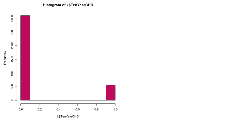
It’s a good practice to always review the class distribution of our dataset first. One way to look at the class distribution is by using a histogram.

hist(k$TenYearCHD, col="maroon")

The histogram shows that the dataset is imbalanced. The ratio of the positive class to the negative class is too low. This situation is very common, especially in medical datasets. Because in reality, the data from positive illness is low, unless in the pandemic case like Covid-19.

This imbalanced dataset will lead to imbalanced accuracy or imbalanced prediction. This means that the prediction will always inclined towards the majority class, in this case, the negative class. You might see a high accuracy number, but don’t be fooled by that number. Because the sensitivity is low. Therefore, we have to combat this imbalanced dataset before going further.

SMOTE

SMOTE stands for Synthetic Minority Oversampling Technique. This technique will help us resolves the imbalanced dataset problem. As the name implies, this technique will be oversampling the minority class in a synthetic way.

smote <- SMOTE(k[,-16], k$TenYearCHD)
new <- smote$data

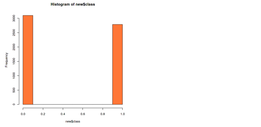
Now our dataset is contained on the new variable, and the label is now on a column named class. We can see in the histogram that our class is now balanced. The number of the data doesn’t have to be exactly the same, but the difference has to be minimum.

hist(new$class, col=”coral”)

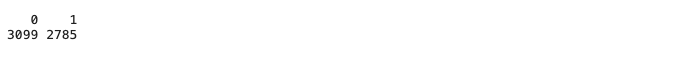
We can also print the number of the data from each class

new$class <- as.numeric(new$class)
table(new$class)

and we can print the percentage like this

prop.table(table(new$class))

Best model selection

The function for model selection in R is regsubsets(), where the Nvmax is the number of predictors. After applying the regsubsets function to the dataset, then we save the summary.

model <- regsubsets(as.factor(class)~.,data=new,nvmax=15)
model.sum <- summary(model)

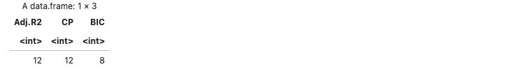
To select the best model, the cross-validated prediction error is used. They are Adjusted R², C_p , and BIC.

Adj.R2 <- which.max(model.sum$adjr2)
CP <- which.min(model.sum$cp)
BIC <- which.min(model.sum$bic)
data.frame(Adj.R2, CP, BIC)

Here we get the results from the three metrics. Adjusted R²and C_p shows the same result, whereas the BIC show different. The best model from Adjusted R²is the model with a higher number. While C_p and BIC show the best model where the result is minimum.

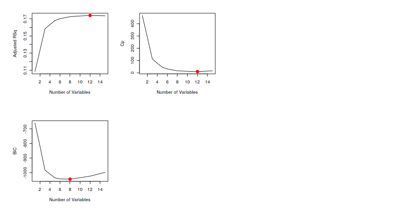
We also can plot the number of predictors to better see the result from regsubsets().

par(mfrow=c(2,2))
plot(model.sum$adjr2,xlab="Number of Variables",ylab="Adjusted RSq",type="l")
points(Adj.R2,model.sum$adjr2[Adj.R2], col="red",cex=2,pch=20)
plot(model.sum$cp,xlab="Number of Variables",ylab="Cp",type="l")
points(CP,model.sum$cp[CP],col="red",cex=2,pch=20)
plot(model.sum$bic,xlab="Number of Variables",ylab="BIC",type="l")
points(BIC,model.sum$bic[BIC],col="red",cex=2,pch=20)

The red dots show the number of predictors which produce the best model from each metric.

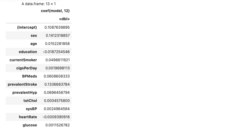
These are the best twelve predictors. We can show them via the coefision function.

The best linear regression model can be achieved using these twelve predictors. It means that we can get better or the same regression result using just these twelve predictors instead of fifteen.

as.data.frame(coef(model, 12))

Compare the linear regression model

Now let’s compare the linear regression model using all the predictors and using best subset selection. First, we do a linear regression using all the predictors.

lm.fit.before <- lm(class~., data=new)

lm.probs.before <- predict(lm.fit.before, type="response")

lm.pred.before <- rep(0, length(lm.probs.before))

lm.pred.before[lm.probs.before > 0.5] <- 1

table(lm.pred.before, new$class)

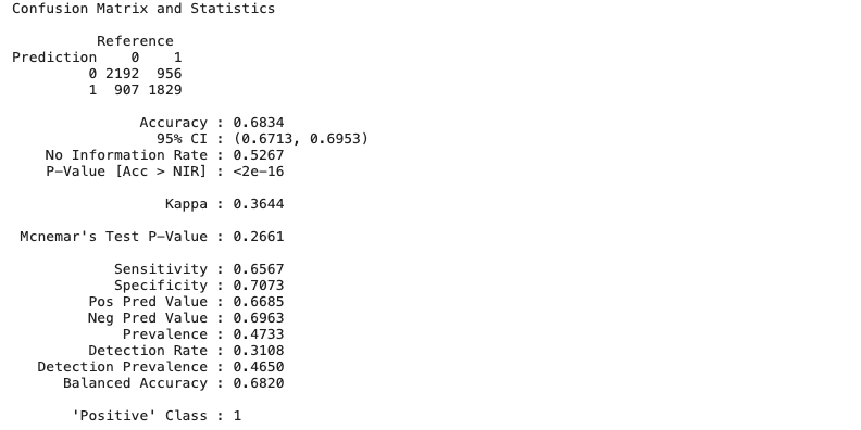
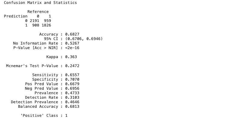
Further, we can print the confusion matrix to get a better insight. Here we get 68% accuracy before the implementation of the best subset selection.

Other than accuracy, we can also look at the sensitivity and specificity measurement. We get the number that isn’t too far apart between the two. This happens because we have implemented SMOTE before.

lm.before <- confusionMatrix(data =  as.factor(lm.pred.before), reference = as.factor(new$class), positive="1")
lm.before

Then, we do a linear regression using twelve predictors from the best subset selection.

lm.fit.after <- lm(class~sex+age+education+currentSmoker+cigsPerDay+BPMeds+prevalentStroke+prevalentHyp+totChol+sysBP+heartRate+glucose, data=new)
lm.probs.after <- predict(lm.fit.after, type="response")
lm.pred.after <- rep(0, length(lm.probs.after))
lm.pred.after[lm.probs.after > 0.5] <- 1
table(lm.pred.after, new$class)

The result is the accuracy also 68%, the same with all fifteen predictors. The same accuracy acquired using fewer predictors.

lm.after <- confusionMatrix(data =  as.factor(lm.pred.after), reference = as.factor(new$class), positive="1")
lm.after

Short Author Bio

My name is Muhammad Arnaldo, a machine learning and data science enthusiast. Currently a master’s student of computer science in Indonesia.