This article was published as a part of the Data Science Blogathon.
Introduction to Pyspark
Spark is an open-source framework for big data processing. It was originally written in scala and later on due to increasing demand for machine learning using big data a python API of the same was released. So, Pyspark is a Python API for spark. It integrates the power of Spark and the simplicity of Python for data analytics. Pyspark can effectively work with spark components such as spark SQL, Mllib, and Streaming that lets us leverage the true potential of Big data and Machine Learning.
In this article, we are going to build a classification pipeline for penguin data. We will discuss dealing with missing data, and scaling and transforming data with the help of the pipeline module of Pyspark.
Initiate a Spark Session
Spark sessions are the entry point to every underlying spark functionality. It lets us create and use RDDs, Dataframes and Datasets. So, to work with the spark it is imperative to initiate a spark session. In Python, we can do this by using the builder pattern mentioned below.
from pyspark.sql import SparkSession
spark = SparkSession
     .builder
     .appName('classification with pyspark')
     .config("spark.some.config.option", "some-value")
     .getOrCreate()
Read Data
Now that a spark session has been created we will now be able to read our data through the following code snippet.
dt = spark.read.csv('D:Data Setspenguins_size.csv',  header=True)
dt.show(5)
+-------+---------+----------------+---------------+-----------------+-----------+------+
|species|   island|culmen_length_mm|culmen_depth_mm|flipper_length_mm|body_mass_g|   sex|
+-------+---------+----------------+---------------+-----------------+-----------+------+
| Adelie|Torgersen|            39.1|           18.7|              181|       3750|  MALE|
| Adelie|Torgersen|            39.5|           17.4|              186|       3800|FEMALE|
| Adelie|Torgersen|            40.3|             18|              195|       3250|FEMALE|
| Adelie|Torgersen|              NA|             NA|               NA|         NA|    NA|
| Adelie|Torgersen|            36.7|           19.3|              193|       3450|FEMALE|
+-------+---------+----------------+---------------+-----------------+-----------+------+
only showing top 5 rows
Print schema to know the type of data we have in our dataset.
dt.printSchema()
output: root
 |-- species: string (nullable = true)
 |-- island: string (nullable = true)
 |-- culmen_length_mm: string (nullable = true)
 |-- culmen_depth_mm: string (nullable = true)
 |-- flipper_length_mm: string (nullable = true)
 |-- body_mass_g: string (nullable = true)
 |-- sex: string (nullable = true)
As you can observe all the columns are of string type and we can not operate on string data. So, we will be casting the culmen length, depth and flipper length to float and body mass to an integer.
from pyspark.sql.types import IntegerType, FloatType
df = dt.withColumn("culmen_depth_mm",dt.culmen_depth_mm.cast(FloatType()))
                   .withColumn("culmen_length_mm",dt.culmen_length_mm.cast(FloatType()))
                    .withColumn("flipper_length_mm",dt.flipper_length_mm.cast('float'))
                     .withColumn("body_mass_g",dt.body_mass_g.cast('int'))
You can cast with both the methods mentioned above.
Let’s see if we got our data cast or not.
df.printSchema()
output:root
 |-- species: string (nullable = true)
 |-- island: string (nullable = true)
 |-- culmen_length_mm: float (nullable = true)
 |-- culmen_depth_mm: float (nullable = true)
 |-- flipper_length_mm: float (nullable = true)
 |-- body_mass_g: integer (nullable = true)
 |-- sex: string (nullable = true)
Handling Missing Values
There are missing values in our dataset let’s see which column has how many missing values.
from pyspark.sql.functions import col,isnan, when, count
df.select([count(when(isnan(c) | col(c).isNull() | col(c).contains('NA'), c)).alias(c) for c in df.columns]).show()
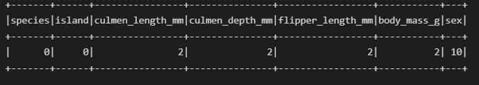
The sex column has missing values but they are in string format so we use contains() alongside IsNull().
Find out rows with missing values
df.where(col('sex').contains('NA')).show()
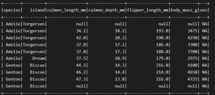
Now, we will create a dataset without any missing values.
df_new = df.where(df.sex != 'NA')
df_new.show(10)
+-------+---------+----------------+---------------+-----------------+-----------+------+
|species|   island|culmen_length_mm|culmen_depth_mm|flipper_length_mm|body_mass_g|   sex|
+-------+---------+----------------+---------------+-----------------+-----------+------+
| Adelie|Torgersen|            39.1|           18.7|            181.0|       3750|  MALE|
| Adelie|Torgersen|            39.5|           17.4|            186.0|       3800|FEMALE|
| Adelie|Torgersen|            40.3|           18.0|            195.0|       3250|FEMALE|
| Adelie|Torgersen|            36.7|           19.3|            193.0|       3450|FEMALE|
| Adelie|Torgersen|            39.3|           20.6|            190.0|       3650|  MALE|
| Adelie|Torgersen|            38.9|           17.8|            181.0|       3625|FEMALE|
| Adelie|Torgersen|            39.2|           19.6|            195.0|       4675|  MALE|
| Adelie|Torgersen|            41.1|           17.6|            182.0|       3200|FEMALE|
| Adelie|Torgersen|            38.6|           21.2|            191.0|       3800|  MALE|
| Adelie|Torgersen|            34.6|           21.1|            198.0|       4400|  MALE|
+-------+---------+----------------+---------------+-----------------+-----------+------+
only showing top 10 rows
Encoding Categorical Variables
Machine learning algorithms can not work with data that is not numerical so before feeding the data to the algorithm it needs to be transformed into numerical data.
So first, we will separate the column names as per their data type, it makes it easier to work with them.
from collections import defaultdict
data_types = defaultdict(list)
for entry in df.schema.fields:
  data_types[str(entry.dataType)].append(entry.name)
print(data_types)
Output: defaultdict(list,
            {'StringType': ['species', 'island', 'sex'],
             'FloatType': ['culmen_length_mm',
              'culmen_depth_mm',
              'flipper_length_mm'],
             'IntegerType': ['body_mass_g']})
cat_cols = [var for var in data_types["StringType"]]
Next up, we will import Stringindexer which is Scikit Learn Labelencoder equivalent of Pyspark and OneHotEncoder. We will use the pipeline method to conveniently transform data from categorical type to numerical type. One hot encoding will create a sparse vector for each row. For detailed knowledge of different encoding methods visit here.
from pyspark.ml.feature import StringIndexer, OneHotEncoder
stage_string_index = [StringIndexer(inputCol=col, outputCol=col+' string_indexed') for col in cat_cols]
stage_onehot_enc =   [OneHotEncoder(inputCol=col+' string_indexed', outputCol=col+' onehot_enc') for col in cat_cols]
from pyspark.ml import Pipeline
ppl = Pipeline(stages= stage_string_index + stage_onehot_enc)
df_trans = ppl.fit(df_new).transform(df_new)
df_trans.show(10)
+-------+---------+----------------+---------------+-----------------+-----------+------+----------------------+---------------------+------------------+------------------+-----------------+--------------+
|species|   island|culmen_length_mm|culmen_depth_mm|flipper_length_mm|body_mass_g|   sex|species string_indexed|island string_indexed|sex string_indexed|species onehot_enc|island onehot_enc|sex onehot_enc|
+-------+---------+----------------+---------------+-----------------+-----------+------+----------------------+---------------------+------------------+------------------+-----------------+--------------+
| Adelie|Torgersen|            39.1|           18.7|            181.0|       3750|  MALE|                   0.0|                  2.0|               0.0|     (2,[0],[1.0])|        (2,[],[])| (2,[0],[1.0])|
| Adelie|Torgersen|            39.5|           17.4|            186.0|       3800|FEMALE|                   0.0|                  2.0|               1.0|     (2,[0],[1.0])|        (2,[],[])| (2,[1],[1.0])|
| Adelie|Torgersen|            40.3|           18.0|            195.0|       3250|FEMALE|                   0.0|                  2.0|               1.0|     (2,[0],[1.0])|        (2,[],[])| (2,[1],[1.0])|
| Adelie|Torgersen|            36.7|           19.3|            193.0|       3450|FEMALE|                   0.0|                  2.0|               1.0|     (2,[0],[1.0])|        (2,[],[])| (2,[1],[1.0])|
| Adelie|Torgersen|            39.3|           20.6|            190.0|       3650|  MALE|                   0.0|                  2.0|               0.0|     (2,[0],[1.0])|        (2,[],[])| (2,[0],[1.0])|
| Adelie|Torgersen|            38.9|           17.8|            181.0|       3625|FEMALE|                   0.0|                  2.0|               1.0|     (2,[0],[1.0])|        (2,[],[])| (2,[1],[1.0])|
| Adelie|Torgersen|            39.2|           19.6|            195.0|       4675|  MALE|                   0.0|                  2.0|               0.0|     (2,[0],[1.0])|        (2,[],[])| (2,[0],[1.0])|
| Adelie|Torgersen|            41.1|           17.6|            182.0|       3200|FEMALE|                   0.0|                  2.0|               1.0|     (2,[0],[1.0])|        (2,[],[])| (2,[1],[1.0])|
| Adelie|Torgersen|            38.6|           21.2|            191.0|       3800|  MALE|                   0.0|                  2.0|               0.0|     (2,[0],[1.0])|        (2,[],[])| (2,[0],[1.0])|
| Adelie|Torgersen|            34.6|           21.1|            198.0|       4400|  MALE|                   0.0|                  2.0|               0.0|     (2,[0],[1.0])|        (2,[],[])| (2,[0],[1.0])|
+-------+---------+----------------+---------------+-----------------+-----------+------+----------------------+---------------------+------------------+------------------+-----------------+--------------+
only showing top 10 rows
In the above code snippet, we defined a pipeline that takes stage_string_indexer and stage_onehot_enc one after the other. The output column of the first stage is used as the input of the second stage.
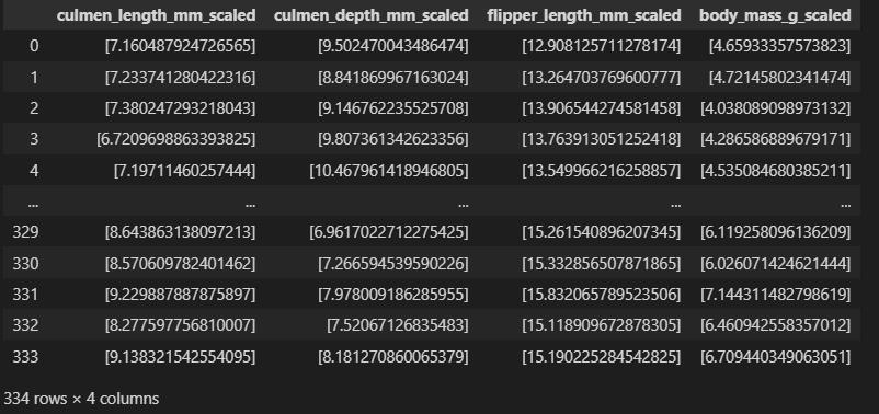
Scaling Parameters
If you observe the data the body mass feature is too large compared to other parameters. And some algorithms are prone to unscaled parameters so it is a good practice to scale the data. Again we will use Pipeline to scale parameters. For this, we will need VectorAssembler and StandardScaler methods.
*VectorAssembler creates a single feature vector out of the given list of columns.
from pyspark.ml.feature import StandardScaler, VectorAssembler
assembler = [VectorAssembler(inputCols=[col], outputCol=col+'_vec') for col in ['culmen_length_mm','culmen_depth_mm','flipper_length_mm','body_mass_g']]
scale = [StandardScaler(inputCol=col+'_vec', outputCol=col+'_scaled') for col in ['culmen_length_mm','culmen_depth_mm','flipper_length_mm','body_mass_g']]
pipe = Pipeline(stages = assembler + scale)
df_scale = pipe.fit(df_trans).transform(df_trans)
df_scale.toPandas().iloc[:,-4:]
Classification Modeling
In this section, we are going to define a pipeline using pyspark that takes care of the classification modelling that we intend to perform. For this article, we will be using a random forest classifier. So, let’s get to the coding part.
train_set, test_set =df_scale.randomSplit([0.75,0.25])
 pyspark.ml.classification import RandomForestClassifier
features = VectorAssembler(inputCols=[ 'island onehot_enc', 'sex onehot_enc',
                                        'culmen_length_mm_scaled','culmen_depth_mm_scaled','flipper_length_mm_scaled',
                                         'body_mass_g_scaled'], outputCol='features')
model_rf = RandomForestClassifier(featuresCol='features', labelCol='species string_indexed')
pipe_lr = Pipeline(stages = [features, model_rf])
In the above code snippet, we defined a vector assembler with selected columns as input from our dataset. Next, we defined our Random Forest classifier with a label column species string_indexed from our already scaled dataset.
Next up, we will define the parameter grid for our pipeline. This is essential for hyperparameter tuning.
from pyspark.ml.tuning import CrossValidator, ParamGridBuilder
from pyspark.ml.evaluation import MulticlassClassificationEvaluator
evaluator = MulticlassClassificationEvaluator(predictionCol='prediction', labelCol='species string_indexed')
parameters = ParamGridBuilder()
            .addGrid(model_rf.bootstrap, [True,False])
            .addGrid(model_rf.maxDepth, [5,10,20,30])
            .build()
cv = CrossValidator(estimator=pipe_lr,
                    estimatorParamMaps=parameters,
                    evaluator= evaluator)
In the above code, we first defined our evaluator which is a Multi-class evaluator where again we specified the label column as before. Then we defined our parameter grid with different model parameters. Finally built the cross validator with a default cross-validation number 3, evaluator, parameter grid and evaluator.
cvModel = cv.fit(train_set)
Let’s find out the best model
cvModel.bestModel.stages[-1]
output: RandomForestClassificationModel: uid=RandomForestClassifier_17983cbf4844, numTrees=20, numClasses=3, numFeatures=8
Training accuracy
cvModel.avgMetrics
Test score summary
predict = cvModel.transform(test_set)

f1 = evaluator.evaluate(predict, {evaluator.metricName:'f1'})

accuracy = evaluator.evaluate(predict, {evaluator.metricName:'accuracy'})

print(f'F1 score:{f1}')

print(f'Accuracy score:{accuracy}')
output: F1 score:0.978494623655914
Accuracy score:0.978494623655914
To get the predicted value we just needed to call transform() on our cvModel.
To make the code even cleaner and more practical you can describe the entire process from the beginning which is encoding categorical variables to classification in a single pipeline. All you need to be careful about is your input and output columns.
Conclusion
Pyspark is one invaluable asset when it comes to machine learning at scale. And to be able to write codes that are neat and easily debuggable is always desired. In this article, we designed a classification pipeline using Pyspark libraries. Some of the key takeaways from the article are below:
- We learnt to load and read datasets with Pyspark
- Performed Encoding of categorical variables with StingIndexer and OneHotEncoder
- We scaled the data using VectorAssembler and StandardScaler
- Finally built a classification pipeline and parameter grid for hyperparameter tuning.
So, this was all about building a machine learning pipeline with Pyspark.
I hope, you liked the article.
The media shown in this article is not owned by Analytics Vidhya and is used at the Author’s discretion.
Meet your author Sunil kumar Dash, a developer and a writer. Has diverse interests in tech, pop culture, wellness, philosophy and Anime. Exploring underrated music is his hobby. And loves to doom scroll Twitter when bored.


