This article was published as a part of the Data Science Blogathon.
Introduction
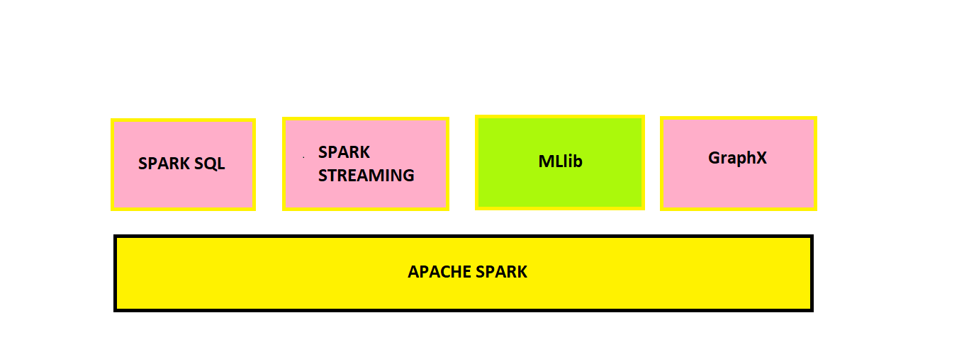
Apache Spark is a fast and general engine used widely for large-scale data processing.
It has several advantages over traditional data processing software. Let us discuss the major advantages below:
-
Speed – Approximately 100 times faster than traditional MapReduce Jobs.
-
Ease of Use – Supports many programming languages like Java, Scala, Python, R, etc.
-
Libraries for SQL Queries, Machine Learning, and Graph Processing applications are present.
-
Parallel Distributed Processing, fault tolerance, scalability, and in-memory computation features make it more powerful.
-
Platform Agnostic- Runs in nearly any environment.
DataFrames Using PySpark
Pyspark is an interface for Apache Spark in Python. Here we will learn how to manipulate dataframes using Pyspark.
Our approach here would be to learn from the demonstration of small examples/problem statements(PS). First, we will write the code and see the output; then, below the output, there will be an explanation of that code.
The dataset is taken from Kaggle: Student Performance DataSet
We will write our code in Google Colaboratory, a rich coding environment from Google. You can install Apache Spark in the local system, also.
(Installation Guide: How to Install Apache Spark)
Instal PySpark
First, we need to install pyspark using the pip command.
!pip install pyspark
import pyspark
Explanation:
The above python codes install and import pyspark in Google Colaboratory.
from pyspark.sql import SparkSession
spark = SparkSession.builder.getOrCreate()
Explanation:
We need to create a spark session to be able to work with dataframes. The above lines of code are exactly doing the same.
Problem Statements (PS)
PS 1. Load the csv file into a dataframe
df=spark.read.csv("StudentsPerformance.csv",header=True,inferSchema=True)
df.show(5)
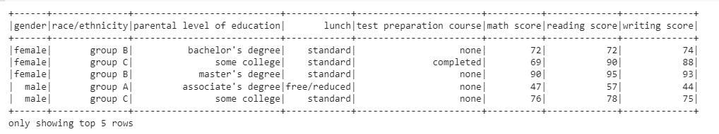
Explanation :
Header -> This parameter indicates whether we want to consider the first row as headers of the columns. Here True means we want the first row as headers.
inferSchema -> It tells the spark function to deduce the datatype(float, int etc.) of the columns in the data.
.show(5) -> Prints/Outputs our dataframe in neat and readable format. Inside the bracket, 5 indicates the number of rows we intend to see, which is 5 in this case.
df.columns
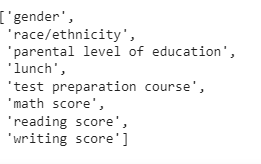
Explanation :
.columns -> This helps us to view the column names of the dataframe.
df.printSchema()
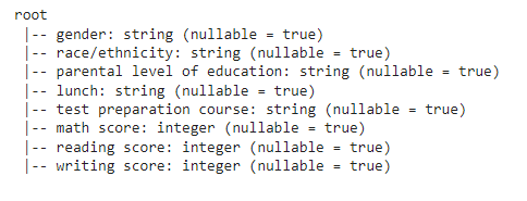
Explanation:
printSchema -> It helps us to view the datatypes of the columns of our DataFrame
nullable=true -> It indicates that the field cannot contain null values.
PS 2. Select an output few values/rows of the math score column
df.select('math score').show(5)

PS 3: Select and output a few values/rows of math score, reading score, and writing score columns
df.select('math score','reading score','writing score').show(5)

PS 4: Create a new column by converting the math scores out of 200 (currently it’s given out of 100)
df.withColumn("Math_Score_200",2*df["math score"]).show(5)
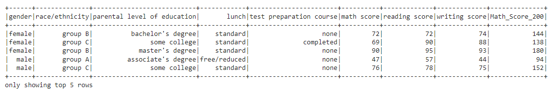
Explanation:
Math_Score_200 is the name of the new column we created whose values are twice the values of math score column i.e, 2*df[“math score”]. So now we have scored out of 200 instead of 100.
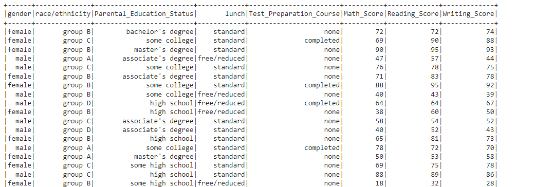
PS 5: Rename the parental level of education column
df.withColumnRenamed("parental level of education","Parental_Education_Status").show(5)

Explanation:
Parental level of education -> old column name
Parental_Education_Status -> new column name
PS 6: Sort the dataframe by reading score values in ascending order
df.orderBy('reading score').show(5)

Explanation:
Note: default is ascending order. So ascending=True is optional
For arranging the dataframe in descending order, we need to type df.orderBy(‘reading score’, ascending=False)
PS 7: Drop race/ethnicity column
df.drop('race/ethnicity').show(5)

PS 8: Show what are all the different education levels of parents
df.select('parental level of education').distinct().collect()
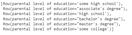
Explanation:
distinct -> It outputs all the distinct values in the column
collect -> it outputs all the data/output generated
PS 9: Find the sum of reading scores for each gender
df.select('gender','reading score').groupBy('gender').sum('reading score').show()
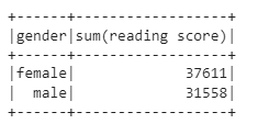
Explanation:
We select our required columns for the task using .select and then group the data by gender using .groupBy and summing the reading scores for each group/category using .sum. Notice the name of the aggregated column is sum(reading score)
PS 10: Filter the dataframe where a reading score greater than 90
df.count()
Explanation:
First, check the total number of rows in the original dataframe. It’s 1000, as seen in the above output.
df.filter(df['reading score']>90).count()
Explanation:
We selected reading score values greater than 90 using the filter function and then counted the number of rows. We can see the number of rows is much less so it filtered and fetched only the rows where the reading score > 90
PS 11: 1. Convert the gender column to uppercase
2. Fetch the lowest marks in the reading score column
from pyspark.sql import functions
Explanation:
pyspark.sql module’s functions are handy to perform various operations on different columns of a dataframe.
print(dir(functions))
Explanation:
We can check what features/functions are available in the functions module using dir
help(functions.upper)
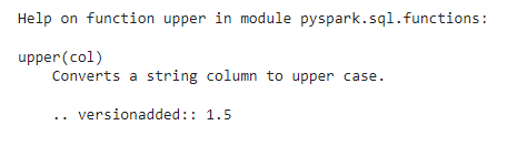
Explanation:
We can check what a particular function does use help
from pyspark.sql.functions import upper,col,min
Explanation:
Imported our required functions for the task.
df.select(min(col('reading score'))).show()
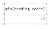
Explanation:
Calculated the minimum value of the reading score column
df.select(col('gender'),upper(col('gender'))).show(5)
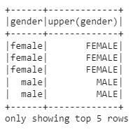
Explanation:
Converted gender to uppercase
PS 12: Rename column names and save them permanently
df=df.withColumnRenamed("parental level of education","Parental_Education_Status")
.withColumnRenamed("test preparation course","Test_Preparation_Course")
.withColumnRenamed("math score","Math_Score")
.withColumnRenamed("reading score","Reading_Score")
.withColumnRenamed("writing score","Writing_Score")
df.show()
Explanation:
Till now, the changes we were doing were temporary. To permanently retain the changes, we need to assign our changes to the same dataframe, i.e., df=df.withColumnsRenamed(..) or if we want to store the changes in a different dataframe, we need to assign them to a different dataframe i.e., df_new=df.withColumnsRenamed(..)
PS 13: Save DataFrame into a .csv file
df.write.csv("table_formed_2.csv",header=True)
Explanation :
We save our dataframe into a file named table_formed_2.csv
header = True -> It indicates that our dataframes header is present.
PS 14: Perform multiple transformations in a single code/query
df.select(df['parental level of education'],df['lunch'],df['math score'])
.filter(df['lunch']=='standard')
.groupBy('parental level of education')
.sum('math score')
.withColumnRenamed("sum(math score)","math score")
.orderBy('math score',ascending=False)
.show()

Explanation:
Notice how we have performed different operations/transformations on the dataframe, one transformation after another.
1st, we select the required col. using .select
2nd, we use .filter to choose lunch type as standard
3rd & 4th, we perform the summation of math score for each level of parent education
5th, we renamed aggregated column sum(math score) to math score
6th, we order/rank our result by math score
7th, we output our result using .show()
PS 15: Create a DataFrame with a single column named DATES which will contain a random date with time information. Create another column side by side with the date 5 days after the date you have chosen initially
from pyspark.sql.functions import to_date, to_timestamp, date_add
Explanation:
Importing required functions
df2=spark.createDataFrame([('2012-11-12 11:00:03',)],['DATES'])
df2.show()

Explanation:
Creating dataframes with a single row containing date & time (format: YYYY-dd-MM HH:mm:ss ) and column name DATES
df3=df2.select(to_date(col('DATES'),'yyyy-dd-MM'),to_timestamp(col('DATES'),'yyyy-dd-MM HH:mm:ss'))
renamed_cols = ['DATE','TIMESTAMP']
df4= df3.toDF(*renamed_cols)
df4.show()
Explanation:
Created dataframes df3 first with two columns, one containing only date info and another containing date & time info. Note that for the latter case, we used the to_timestamp function.
We then created a df4 dataframe from df3 with the same information, but this time added the column names DATE and TIMESTAMP.
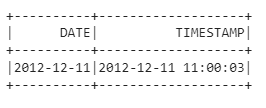
df4.select(col('TIMESTAMP'),date_add(col('TIMESTAMP'),5)).show(1, truncate=False)
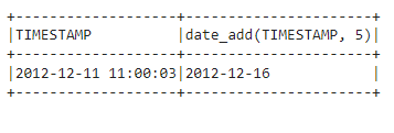
Explanation:
As asked in the PS, we successfully added 5 days to the date. Notice we used the date_add function.
truncate=False -> Indicates to show all the rows and their full content. Thus it helps us to see full data of all a row in a dataframe without truncation.
Conclusion
We can conclude that with improved speed and other advantages, Apache Spark stands out when working with enormous data. Today a lot of data scientists use Python for their daily tasks. Integrating Spark to Python through PySpark is undoubtedly a blessing to them in dealing with large-scale data. Throughout this article, here are the things we have learned:
• Basic Introduction to Apache Spark and its advantages.
• Perform different transformations on dataframe using PySpark with proper explanations.
• In short, PySpark is very easy to implement if we know the proper syntax and have little practice. Extra resources are available below for reference.
PySpark has many more features like using ML Algorithms for prediction tasks, SQL Querying, and Graph Processing, all with straightforward & easily-interpretable syntax like the ones we saw in the above tutorial. I hope you liked my article on DataFrames using Pyspark. Share your views in the comments below.
The media shown in this article is not owned by Analytics Vidhya and is used at the Author’s discretion.
Masters's Student at a University. My area of specialization is Data Science. Interested in doing quality research work in this field. I love to spread the knowledge I learn to the audience through blogs and articles.


