40 Advanced SQL Window Functions Every Data Scientist Must Know(with examples)

In the world of data science, SQL still remains the powerful tool for defining the data, data manipulation, data aggregation and data analysis.

While basic SQL commands are very fundamental, and everyone knows about it. If you want to be the unique in the crowd then you should know advanced features like window functions that can unlock multiple capabilities for complex data transformations and insights. In this article, you will learn about those advanced SQL window functions that you be aware of and how to use them in your project.

Difference between Window Functions and Regular Aggregate Functions

Regular aggregate functions like (SUM(), AVG(), COUNT() without OVER()): These functions collapse rows into summary. It takes a group of rows and return a single summary row. For example: “SELECT SUM(sales) FROM orders gives you total number of sales number.

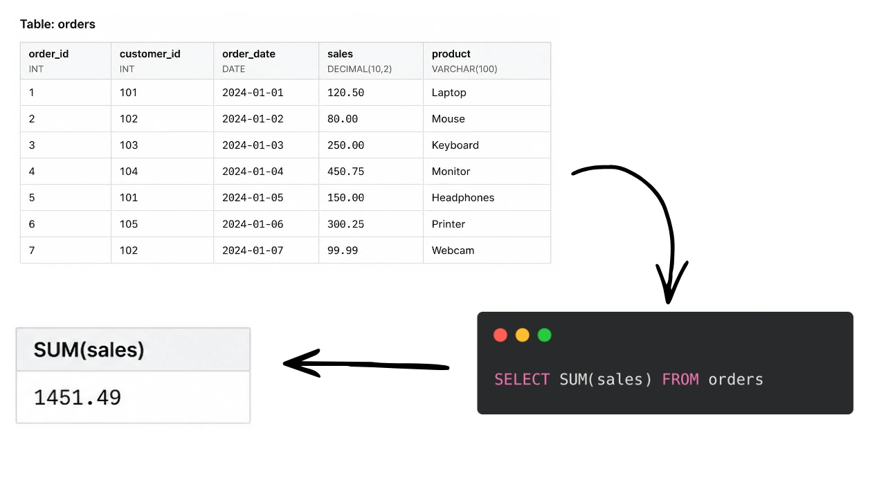
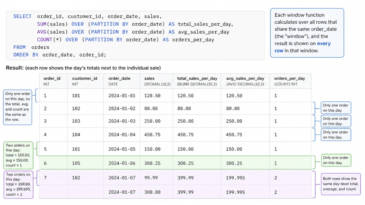
Windows Functions like (SUM(), AVG(), COUNT() with OVER()): These functions also perform calculations on group of rows, but they return a result for every single row in your original data. This means you can see the total sales for the day next to each individual sales that happened on that day.

The Magic OVER() Clause: Defining your window

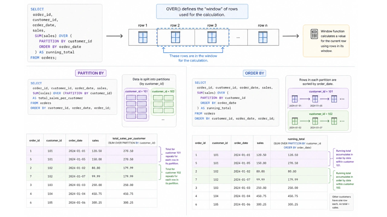
The OVER() clause is the heart of every window function. It tells SQL exactly which rows to include in your window for the calculation. Inside OVER(), you can use a few important keywords:

• PARTITION BY: This is like saying “Group my data by this column”. For example, PARTITION BY customer_id means window function will restart its calculation for each new customer.
• ORDER BY: This tells SQL how to sort the rows with in each group(or the whole dataset if there’s no PARTITION BY). This is super important for functions that care about sequence, like finding the first or next item.

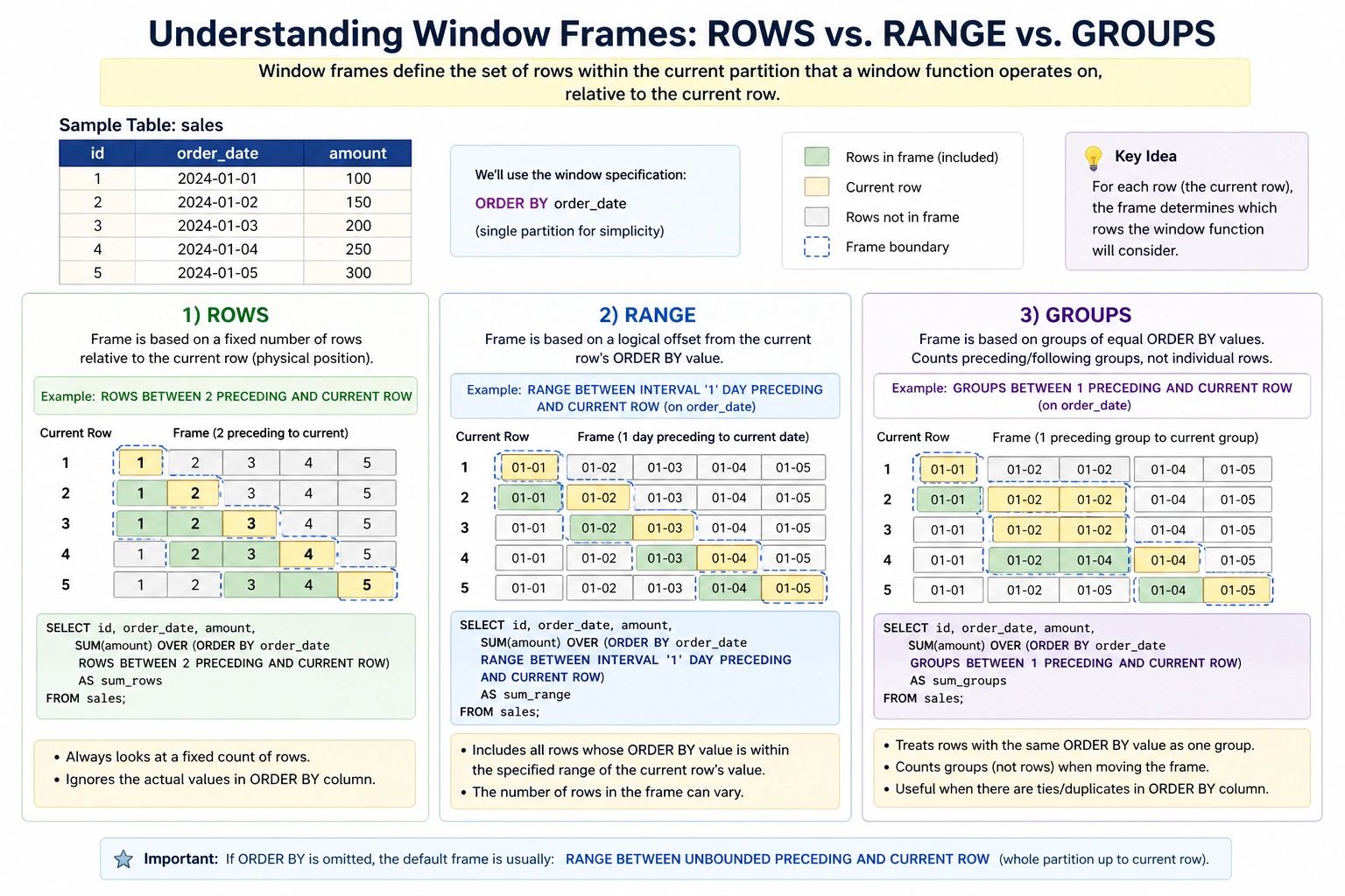
Understanding Window Frames: ROWS vs RANGE vs GROUPS

Window frames specify the subset of rows within the current partition that the window function should operate on. They are defined relative to the current row and are critical for calculations like moving averages or cumulative sums.

• ROWS: Defines the frame based on a fixed number of rows preceding or following the current row. For example, ROWS BETWEEN 2 PRECEDING AND CURRENT ROW includes the current row and the two preceding rows.
• RANGE: Defines the frame based on a logical offset from the current row’s value in the ORDER BY clause. For instance, RANGE BETWEEN 100 PRECEDING AND CURRENT ROW would include all rows whose ORDER BY value is within 100 units of the current row’s value.
• GROUPS: (Less common, but available in some advanced SQL dialects like Oracle) Defines the frame based on a logical group of rows, similar to RANGE but often used with more complex grouping logic.

The Essential Ranking and Numbering Functions

These functions are good for sorting your data and assigning ranks or numbers within groups. They help you quickly find the best, worst or simply count items in a sequence.

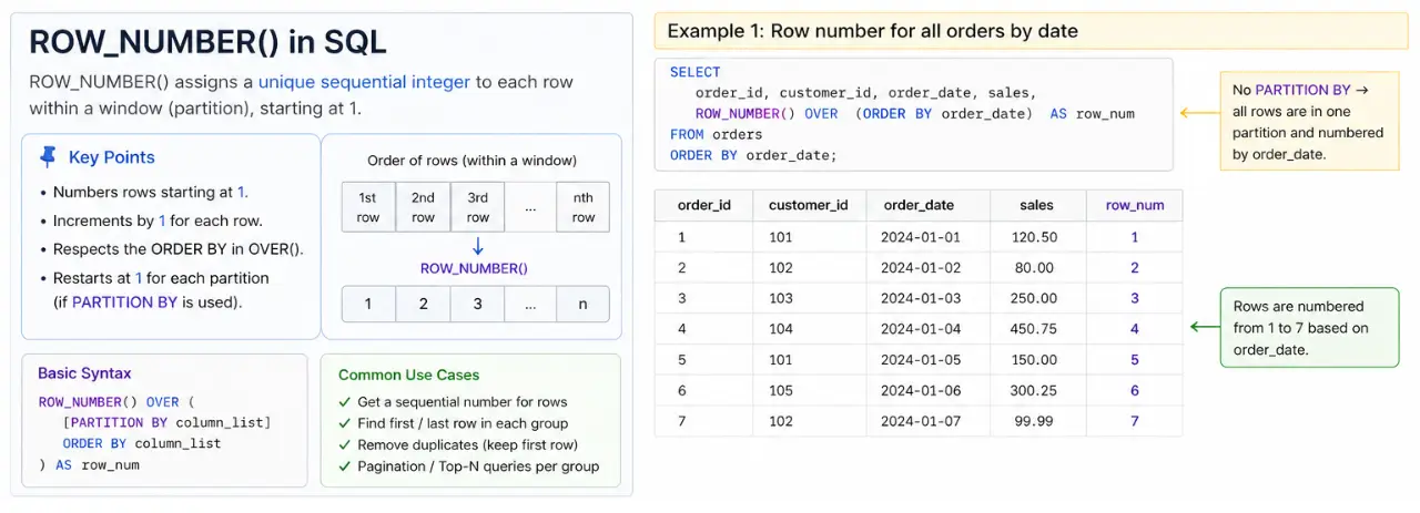
ROW_NUMBER(): Giving Each Row a Unique Number

ROW_NUMBER() assigns a unique, sequential number(starting from 1) to each row within group. It’s perfect when you need a simple, distinct ID for each item based on a specific order.

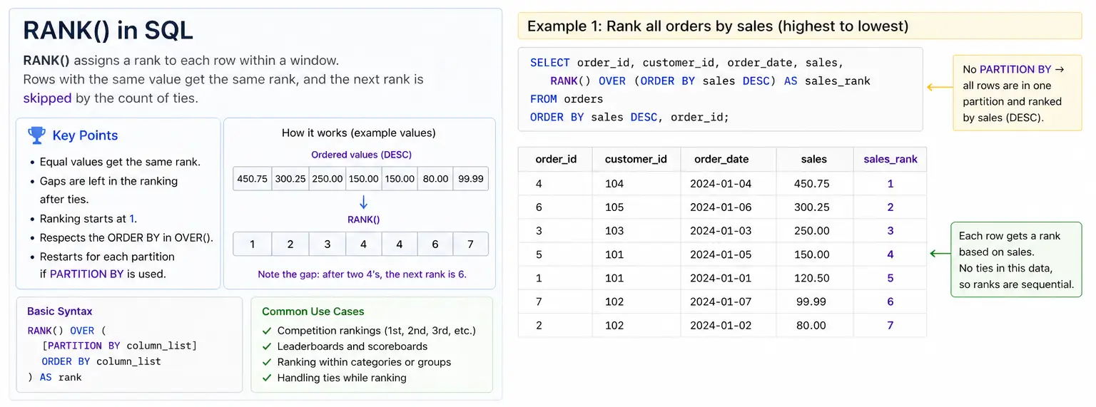
RANK(): Ranking with Gaps for Ties

RANK() gives rank to each row within its group. If two rows have the same value(a “tie”), they get the same rank. The next ranks then “skips” numbers. So if two items are ranked #1, the next item would be #3(skipping #2)

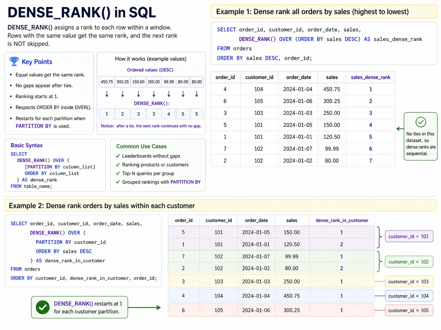
DENSE_RANK(): Ranking Without Gaps

DENSE_RANK() is very similar to RANK() but it doesn’t skip numbers where there are ties. If two items are ranked #1, the next item will be #2(no skipped numbers)

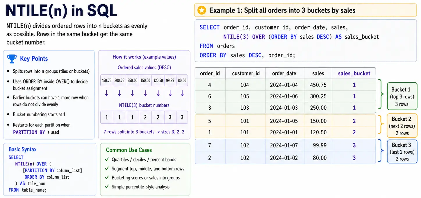
NTILE(n): Dividing into Equal Groups

NTILE(n) divides your rows into “n” equal groups(for equal as possible). It assigns a number from 1 o ‘n’ to each group. This is great for creating segments like quartiles(4 groups), deciles(10 groups) or any other bucket for analysis.

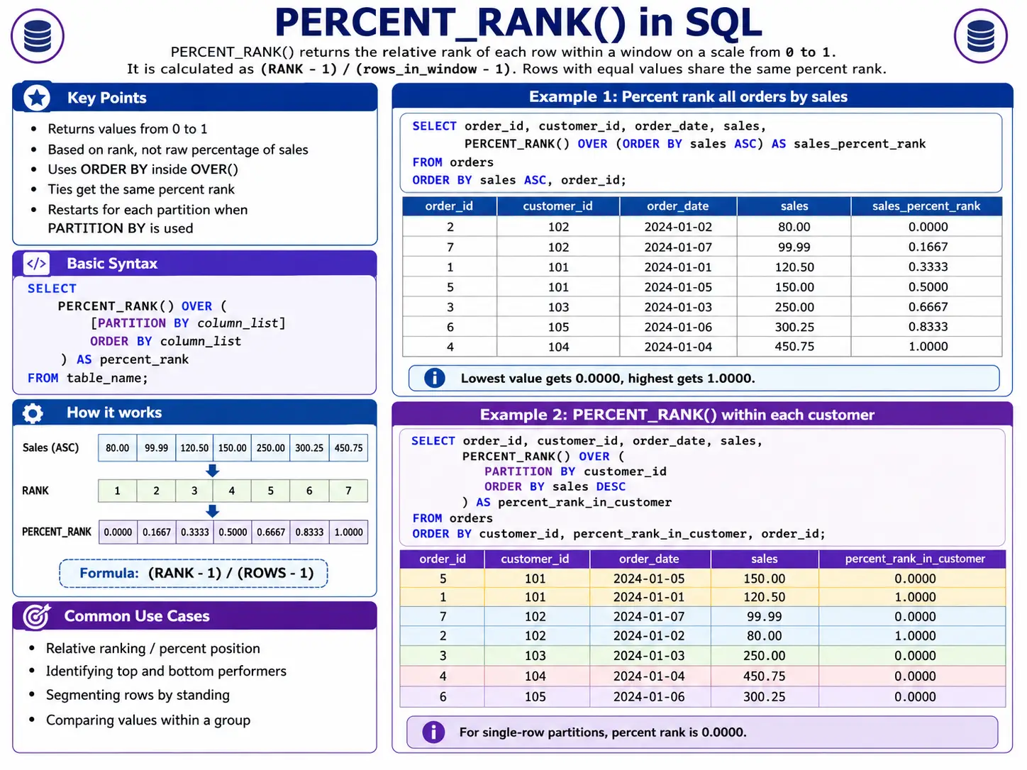
PERCENT_RANK(): Showing Relative Position

PERCENT_RANK() tell you the relative rank of a row within its group as a percentage from 0 to 1. It shows you where a specific item stands compared to all others in its group.
The Essential Ranking and Numbering Functions.

Navigation & Positional Functions

These functions are like time travellers for your data! They let you look at values from rows before or after the current within your window. This is super useful for comparing things over time, like seeing how today’s sales compare to yesterday’s.

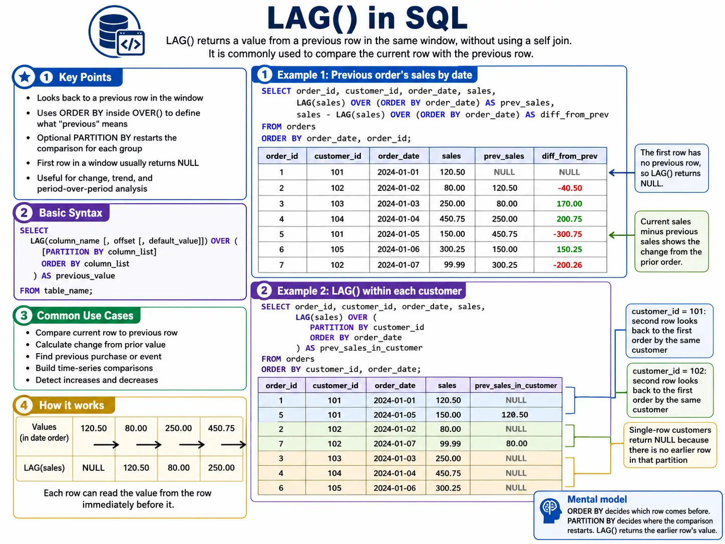
LAG(): Looking Back in Time

LAG() lets you grab a value from a row that came before the current row. You can specify how many rows back you want to look. It’s perfect for calculating things like “change from previous day” or “last known value”

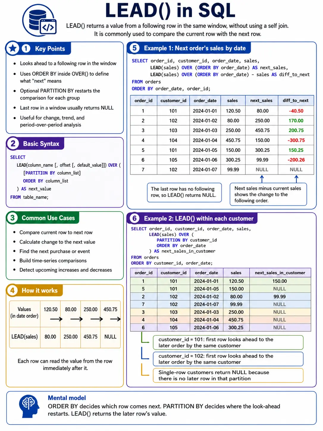
LEAD(): Peeking into the Future

LEAD() is the opposite of LAG(). It lets you grab a value from a row that comes after the current row. This is great for comparing to future values, like “next month’s forecast” or “the event in a sequence”

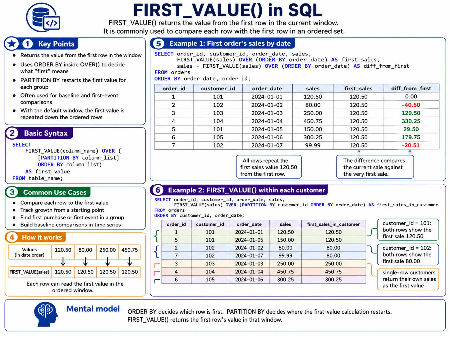
FIRST_VALUE(): Finding the start of the Group

FIRST_VALUE() simply returns the value from the very first row in your current window. This is handy for setting a baseline or comparing everything to the initial state.

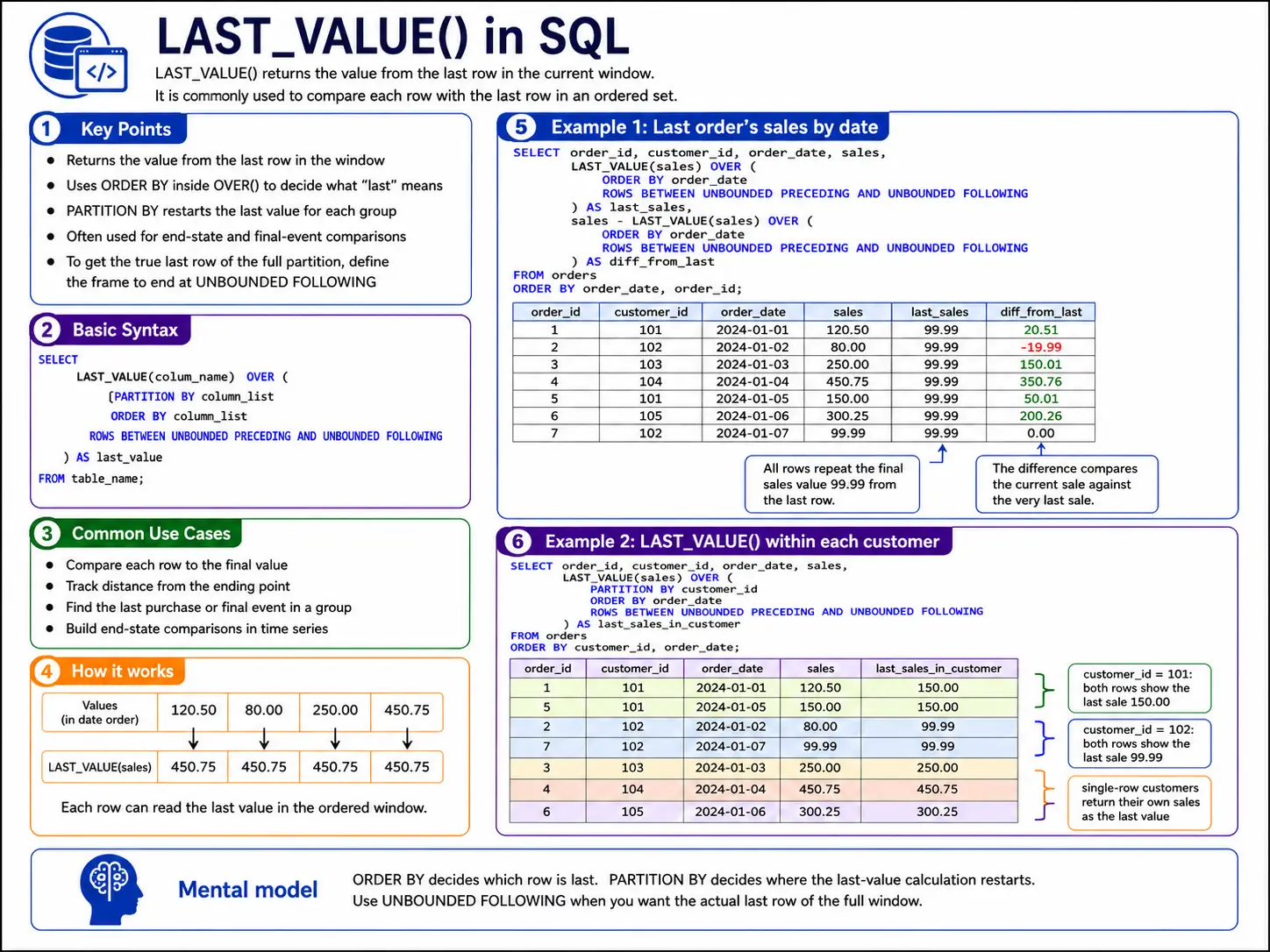
LAST_VALUE(): Finding the End of the Group

LAST_VALUE() returns the value from the last row in your current window. Be careful with this one! By default, the window often only looks up to the current row. To truly get the ‘last value of the entire group‘, you usually need to explicitly tell SQL to look at all rows in the partition using a special frame definition like ‘ROWS BETWEEN UNBOUNDED PRECEDING AND UNBOUNDED FOLLOWING’.

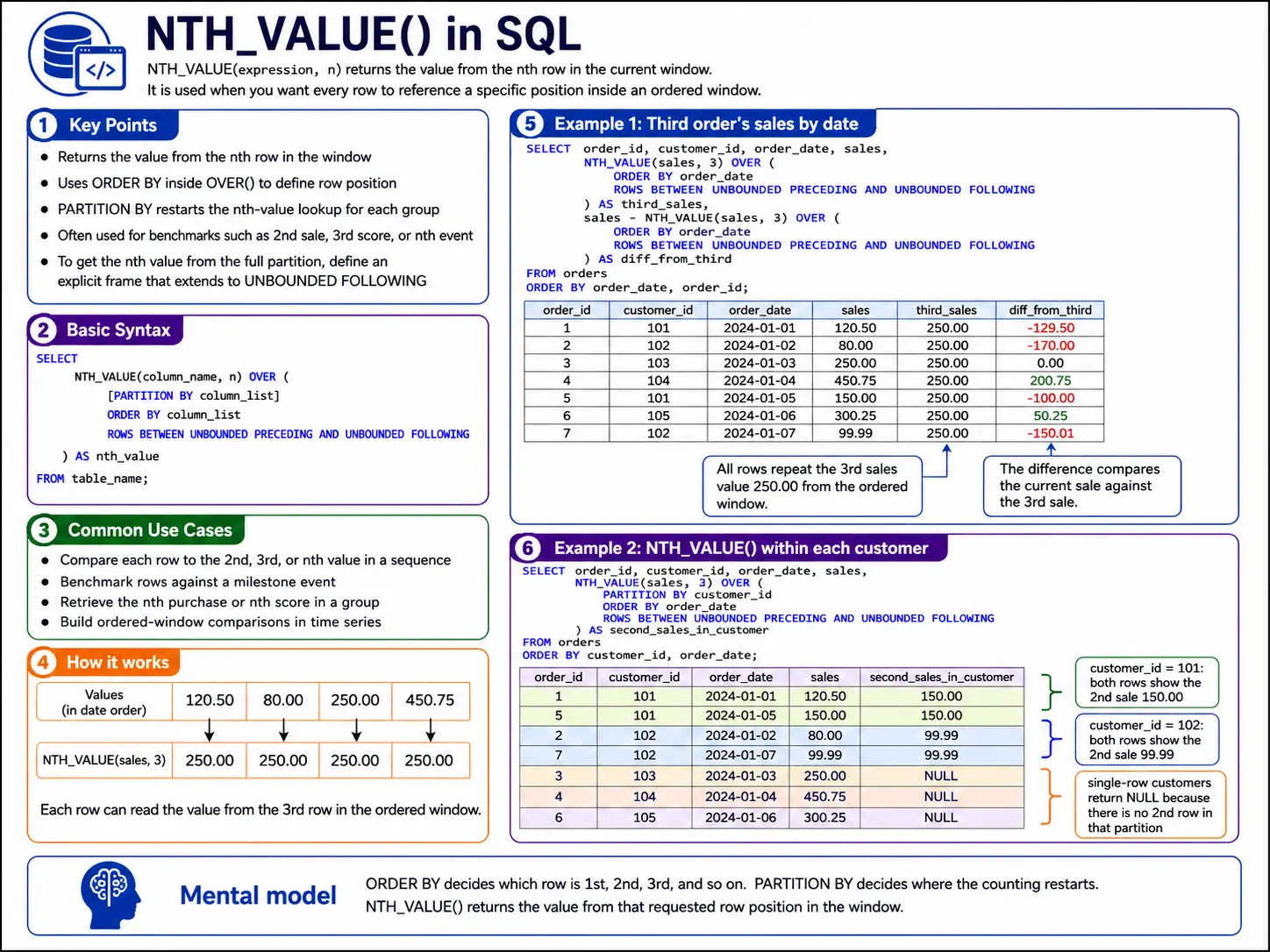
NTH VALUE(expression, n): Picking a specific Row

NTH_VALUE() is more flexible version of FIRST_VALUE() and LAST_VALUE(). It lets you pick the value from the ‘n^th row in your window. So, you could get the 2nd, 3rd, or any specific row’s value.

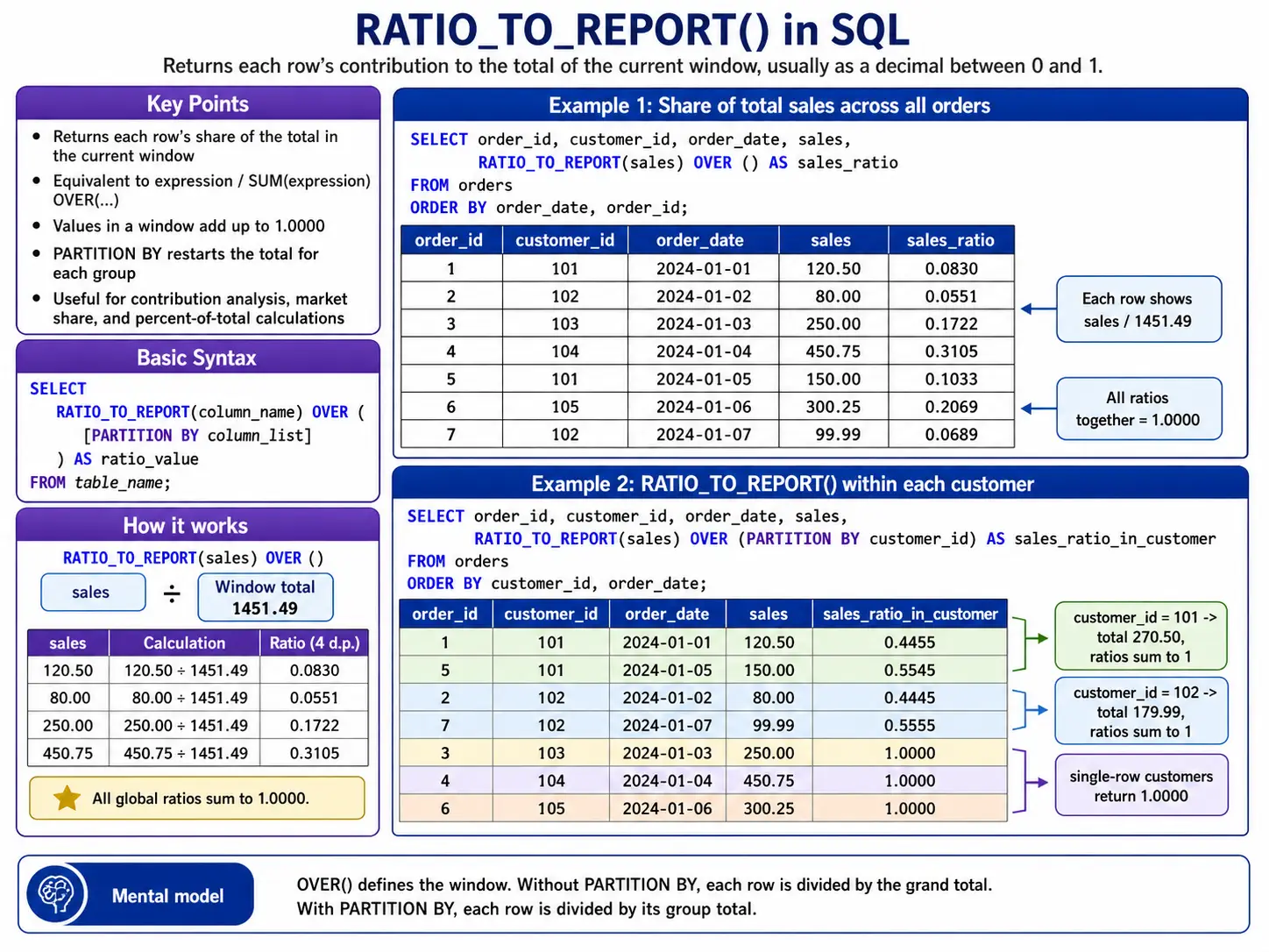
RATIO_TO_REPORT(): Used Specifically in Oracle/BigQuery

RATIO_TO_REPORT() tells you what percentage a specific value contributes to the total sum of its group. It’s great for understanding proportions.

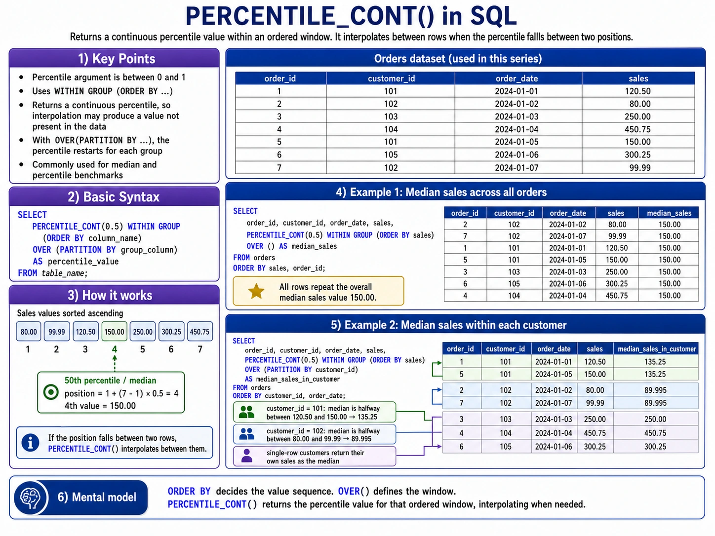
PERCENTILE_CONT(): Finding the Middle Ground

PERCENTILE_CONT() helps you find a percentile (like the median, which is the 50th percentile) in a way that can give you a value between actual data points. It’s like drawing a smooth curve through your data to find the exact point.

Advanced Statistical & Regression Functions

These functions bring serious mathematics power directly into your SQL Queries. They help data scientists to dig deeper into data patterns, measure how spread out data is, and even to find relationships between different columns.

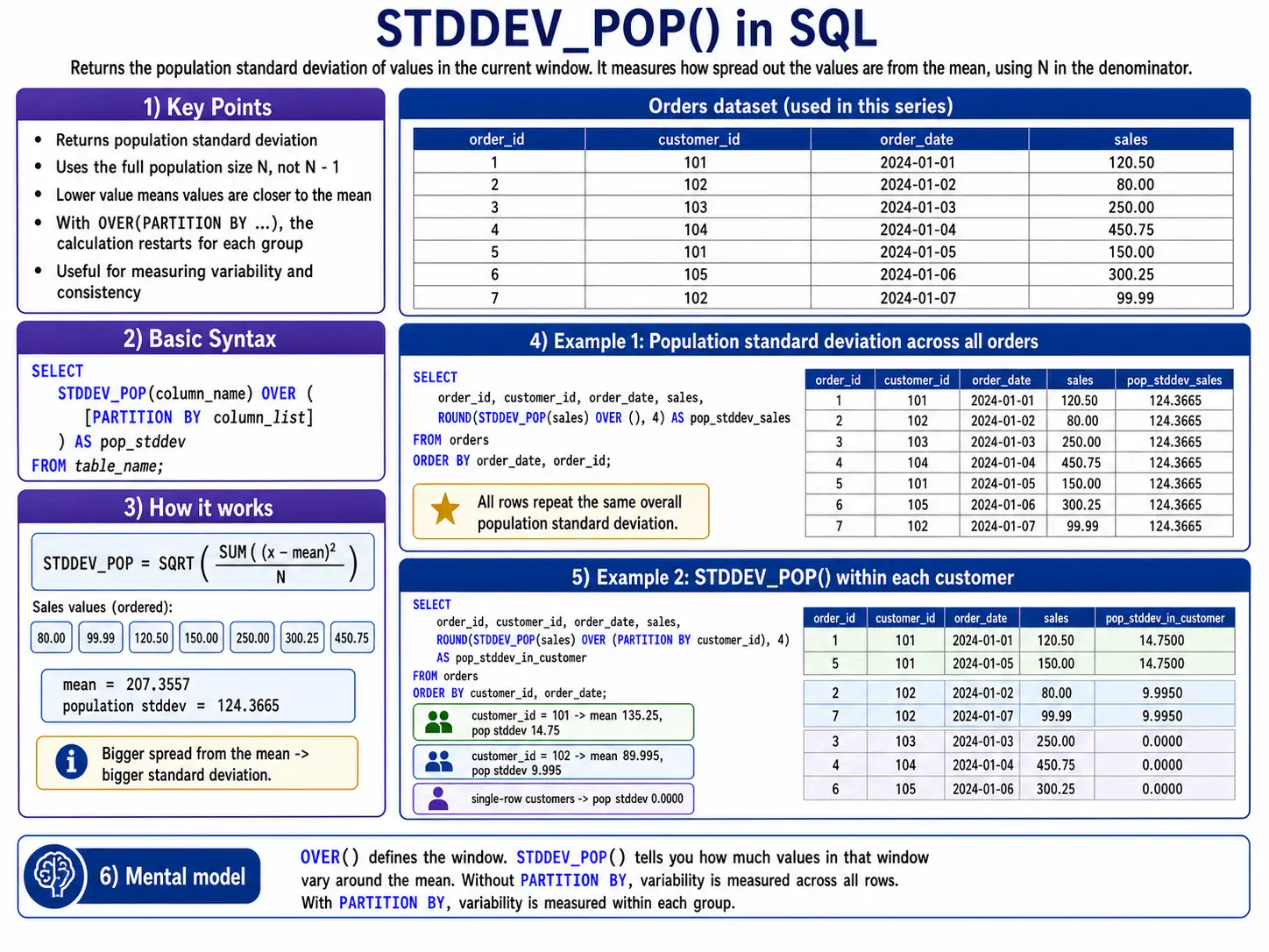
STDDEV_POP(): How Spread Out is My Whole Data?

STDDEV_POP() calculates the standard deviation for an entire group of data (the “population”). It tells you, on average, how far each data point is from the average of the group. A small number means data points are close to the average; a large number means they are more spread out.

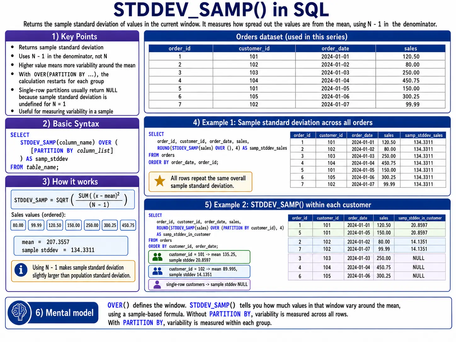
STDDEV_SAMP(): How Spread Out is my Sample Data?

STDDEV_SAMP() is similar to STDDEV_POP(), but it’s used when your data is just a sample of a larger group. It makes a slight adjustment to give a better estimate of the standard deviation of the full population.

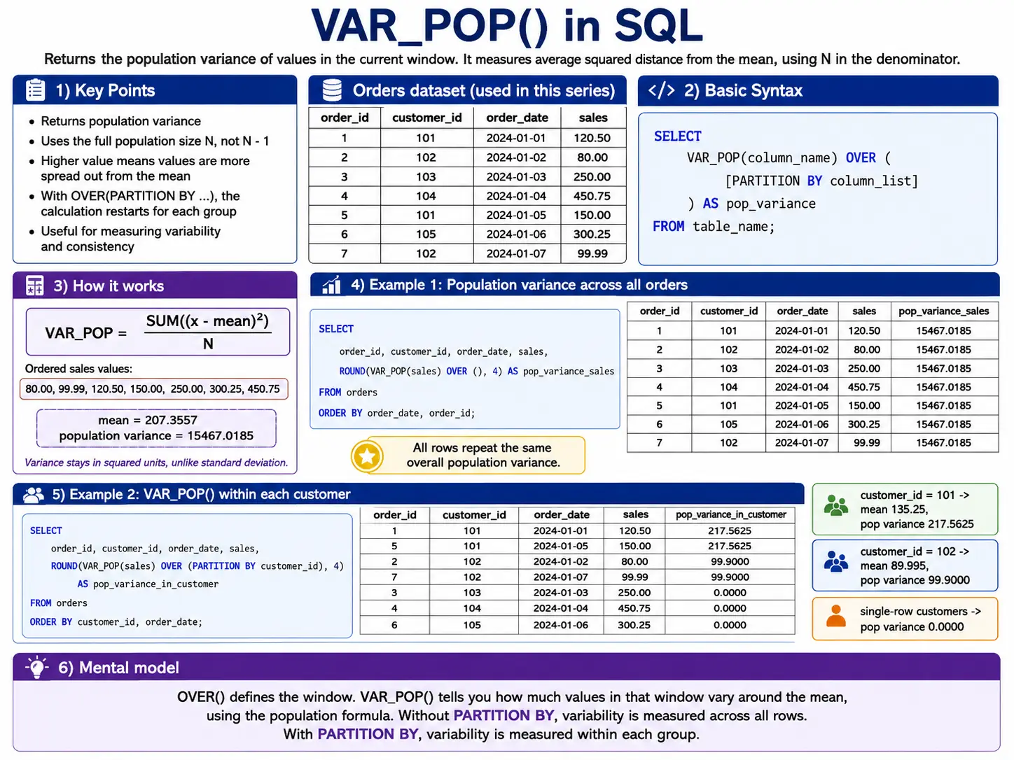
VAR_POP(): The Square of Spread

VAR_POP() calculates the variance for an entire group. Variance is simply the standard deviation squared. It’s another way to measure how spread out your data is.

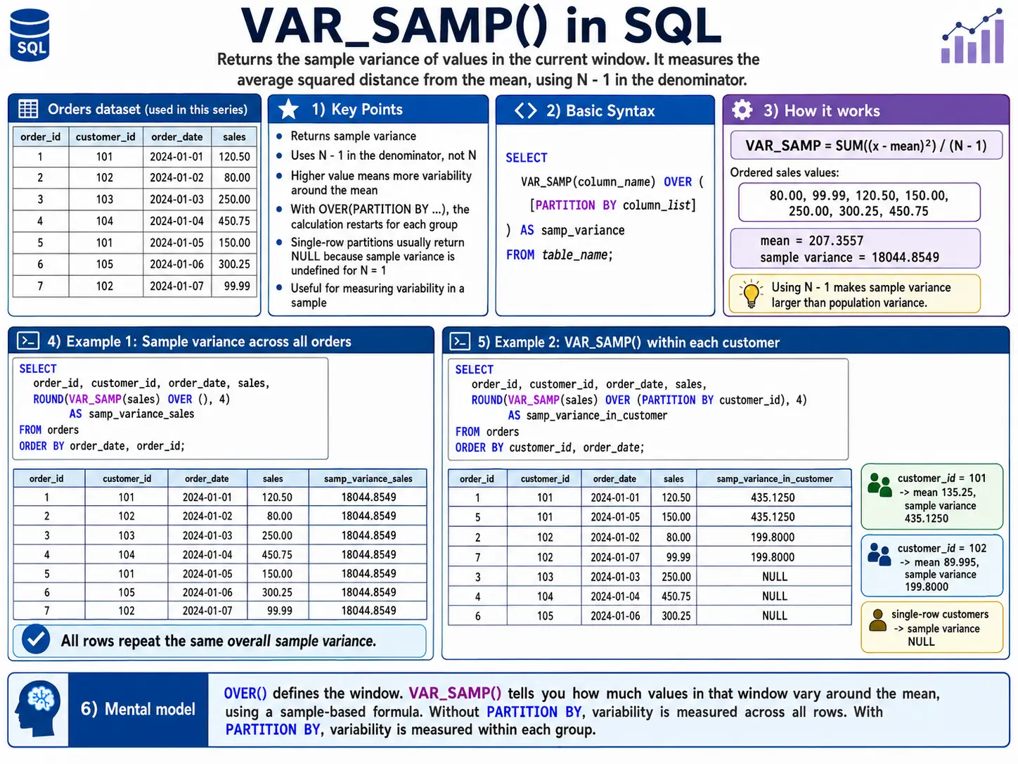
VAR_SAMP(): Sample Variance

Like STDDEV_SAMP(), this calculates the variance when you only have a sample of the data. For Example: Estimate the variance in product weights from a quality control sample.

SELECT
    batch_id,
    product_weight,
    VAR_SAMP(product_weight) OVER (PARTITION BY batch_id) AS sample_weight_variance
FROM
    quality_control;

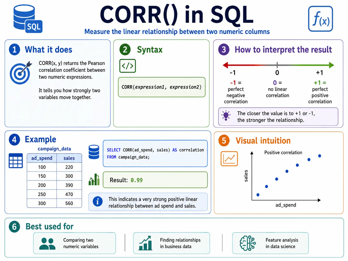
CORR(): Finding Relationships (Correlation)

CORR() measures how strongly two things are related. It gives a number between -1 and 1. A number close to 1 mens as one goes up, the other goes up. Close to -1 means as one goes up, the other goes down. Close to 0 means no real relationship.

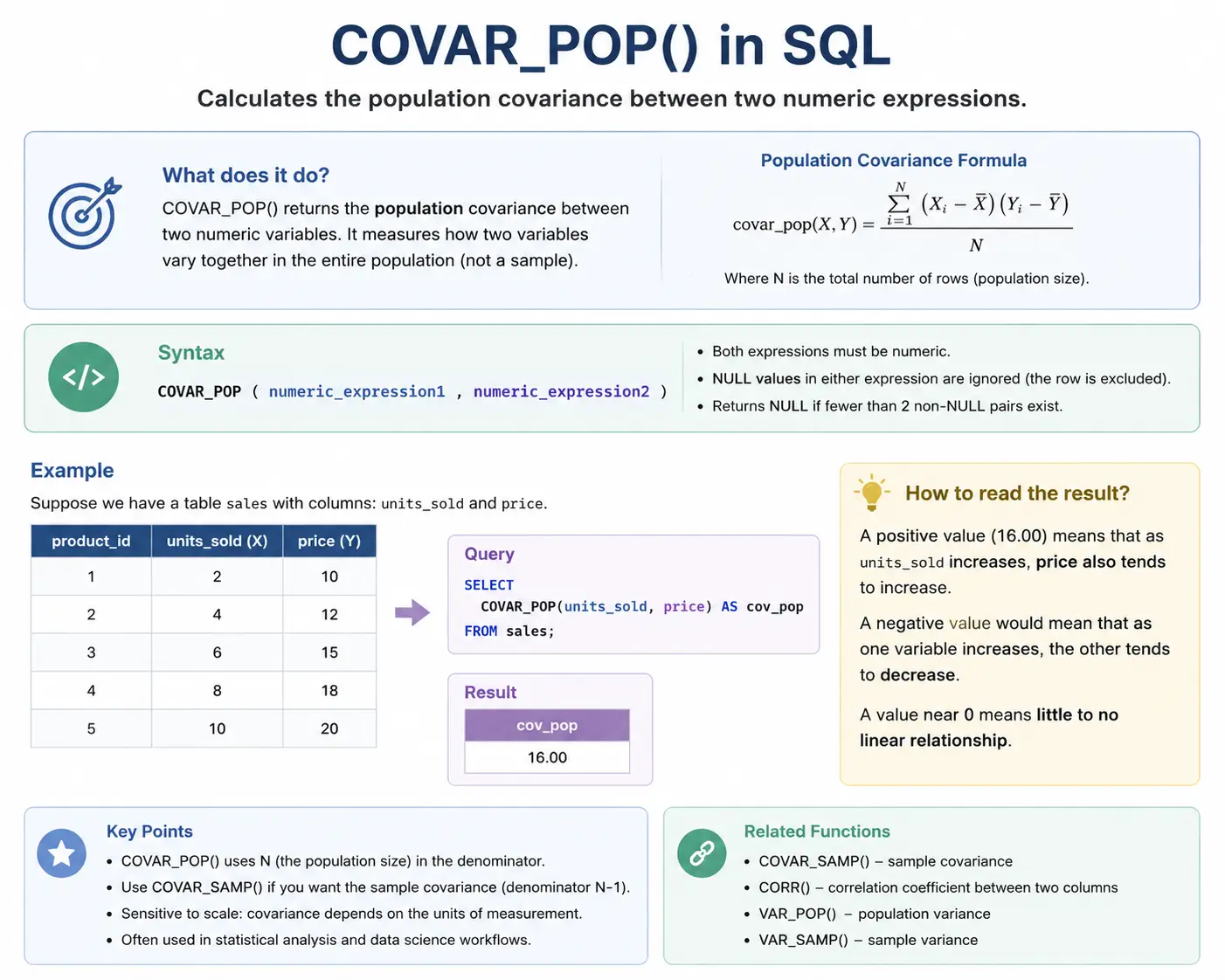
COVAR_POP(): How Things Move Together (Covariance)

COVAR_POP() measures covariance, which is similar to correlation but not scaled between -1 and 1. It tells you the direction of the relationship (positive or negative) between two variables for the whole population.

COVAR_SAMP(): Sample Covariance

This is the sample version of covariance, used when you don’t have all the data.

Example: Estimate the covariance between website load time and bounce rate based on a sample of user sessions.

SELECT
    session_id,
    load_time_ms,
    bounce_flag,
    COVAR_SAMP(load_time_ms, bounce_flag) OVER () AS sample_covariance
FROM
    session_sample;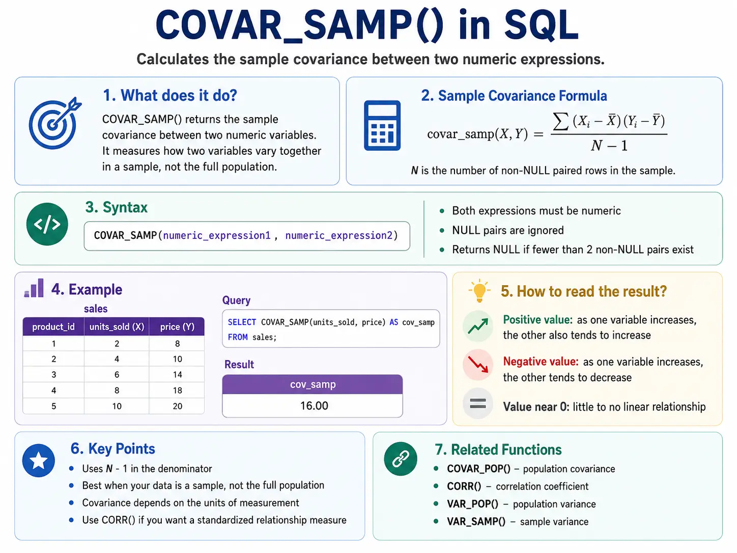

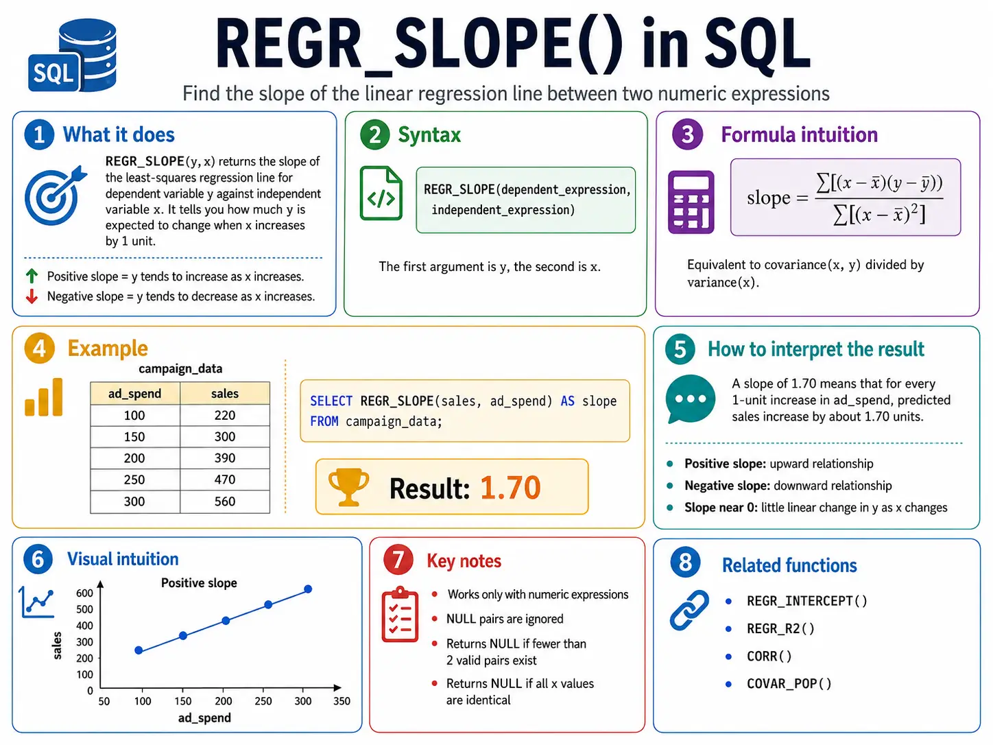
REGR_SLOPE(): Drawing a Trend Line (Slope)

Imagine drawing a “best fit” line through a scatter plot of your data. REGR_SLOPE() tells you the steepness (slope) of that line. It helps you see the general trend.

REGR_INTERCEPT(): Where the Trend Line Starts

REGR_INTERCEPT() tells you where that “best fit” trend line crosses the starting point (the y-axis).

Example: If we project our sales trend backward to month zero, what would the starting sales be?

SELECT
    month_number,
    sales,
    REGR_INTERCEPT(sales, month_number) OVER () AS baseline_sales_estimate
FROM
    monthly_sales;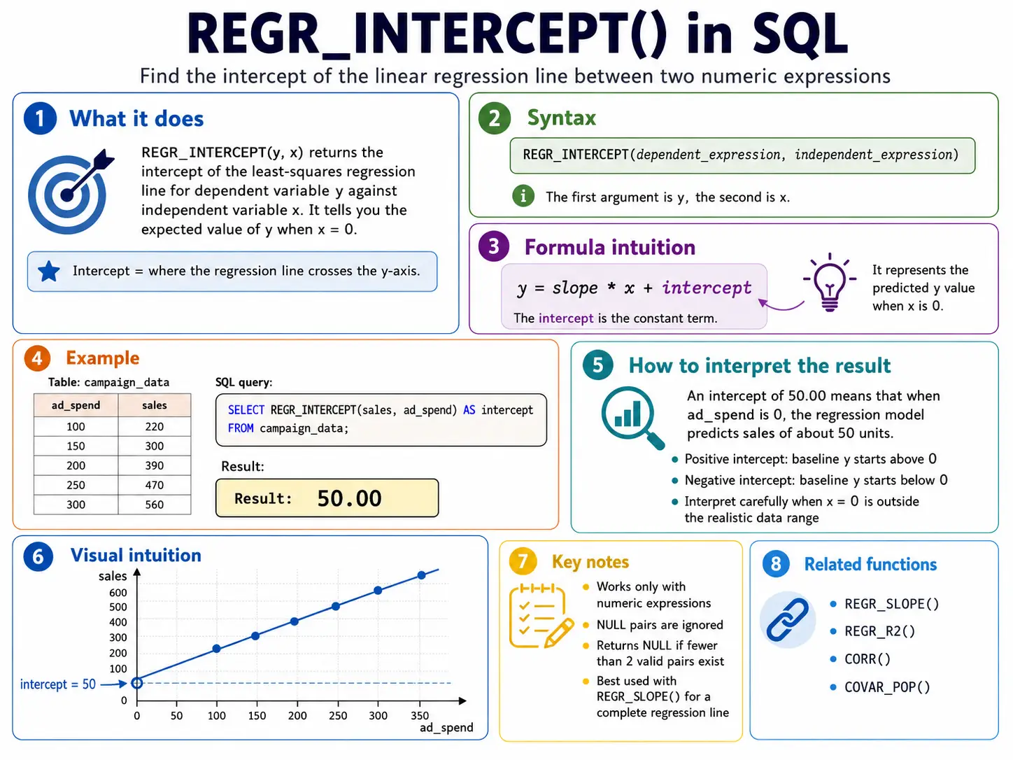

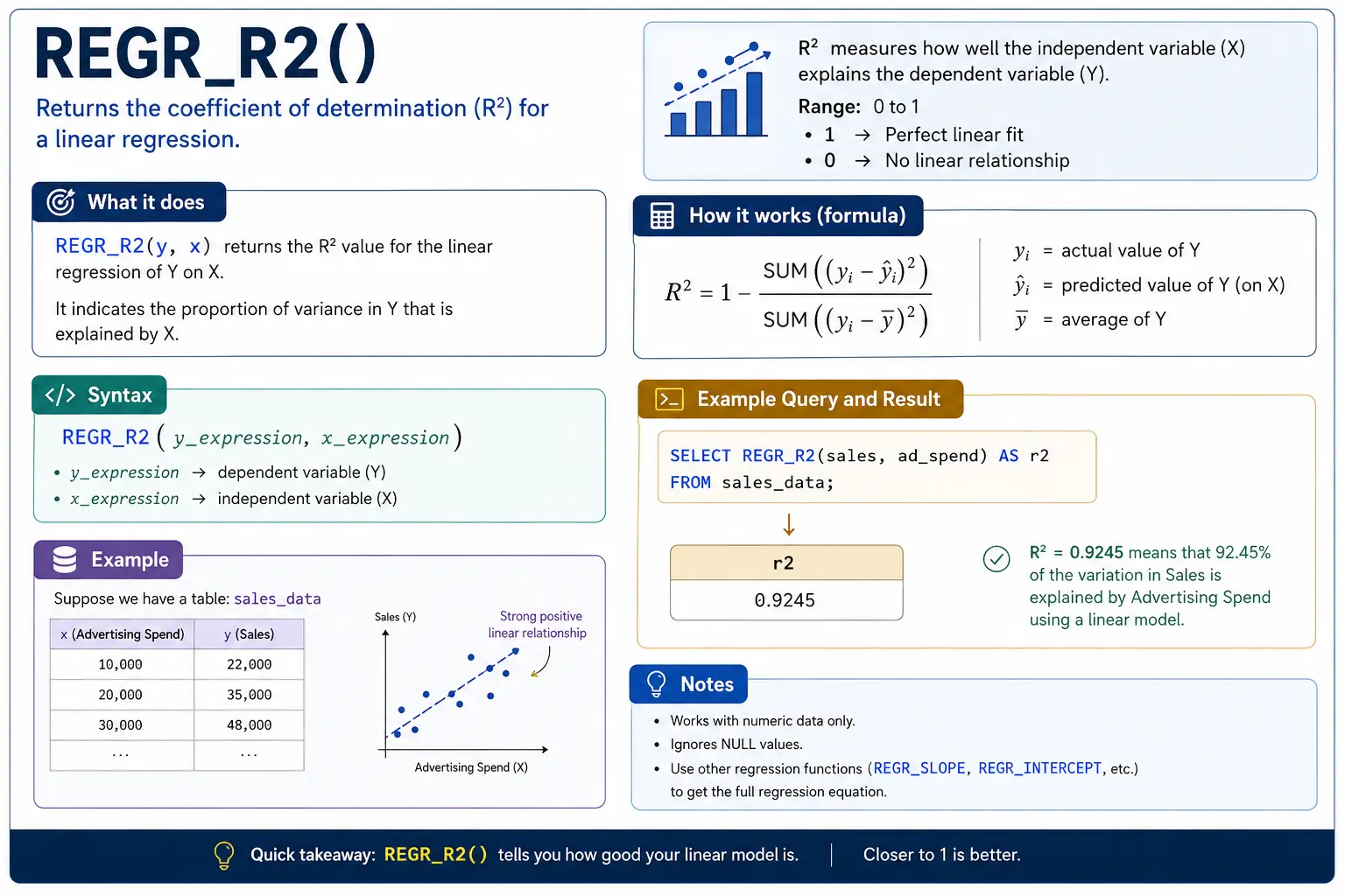
REGR_R2(): How Good is the Trend Line?

REGR_R2() (R-squared) tells you how well your trend line actually fits the data. A score close to 1 means the line is a very good fit; close to 0 means the line doesn’t explain the data well at all.

Distribution & Probability Functions

These functions help you understand the shape of your data. They tell you where a specific value sits compared to everything else, or help you find values at specific points in the distribution.

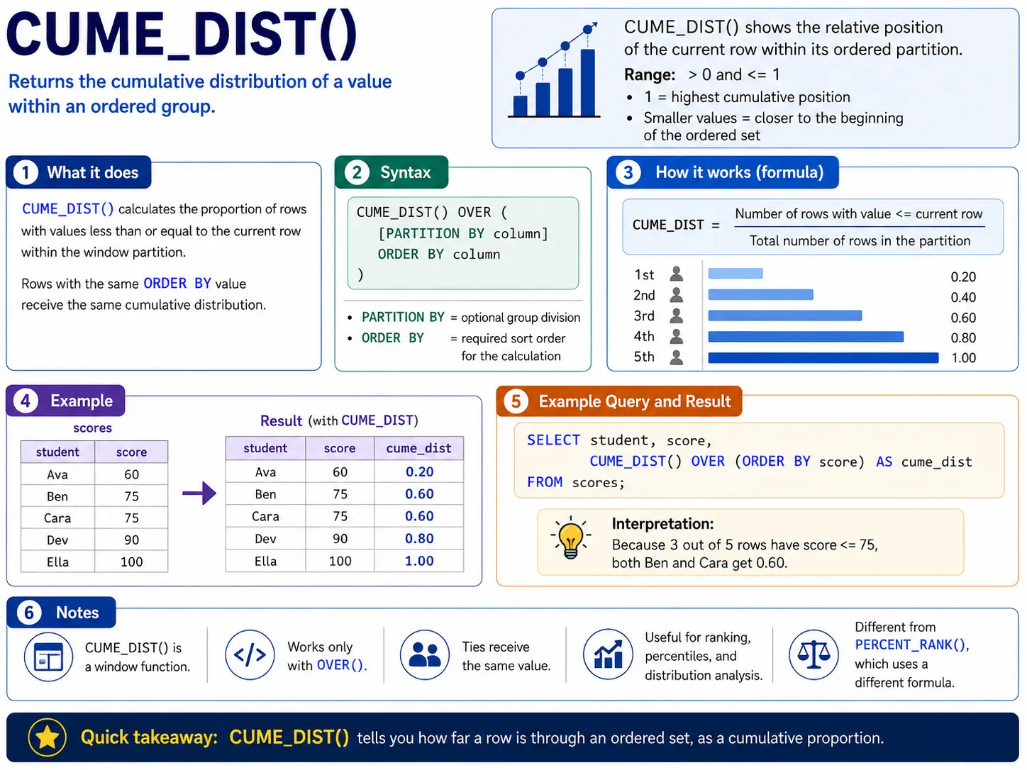
CUME_DIST(): Where Does This Row Stand?

CUME_DIST() tells you what fraction of the rows have a value less than or equal to the current row’s value. It’s like asking, “What percentage of people scored the same or lower than me?” The result is a number between 0 and 1.

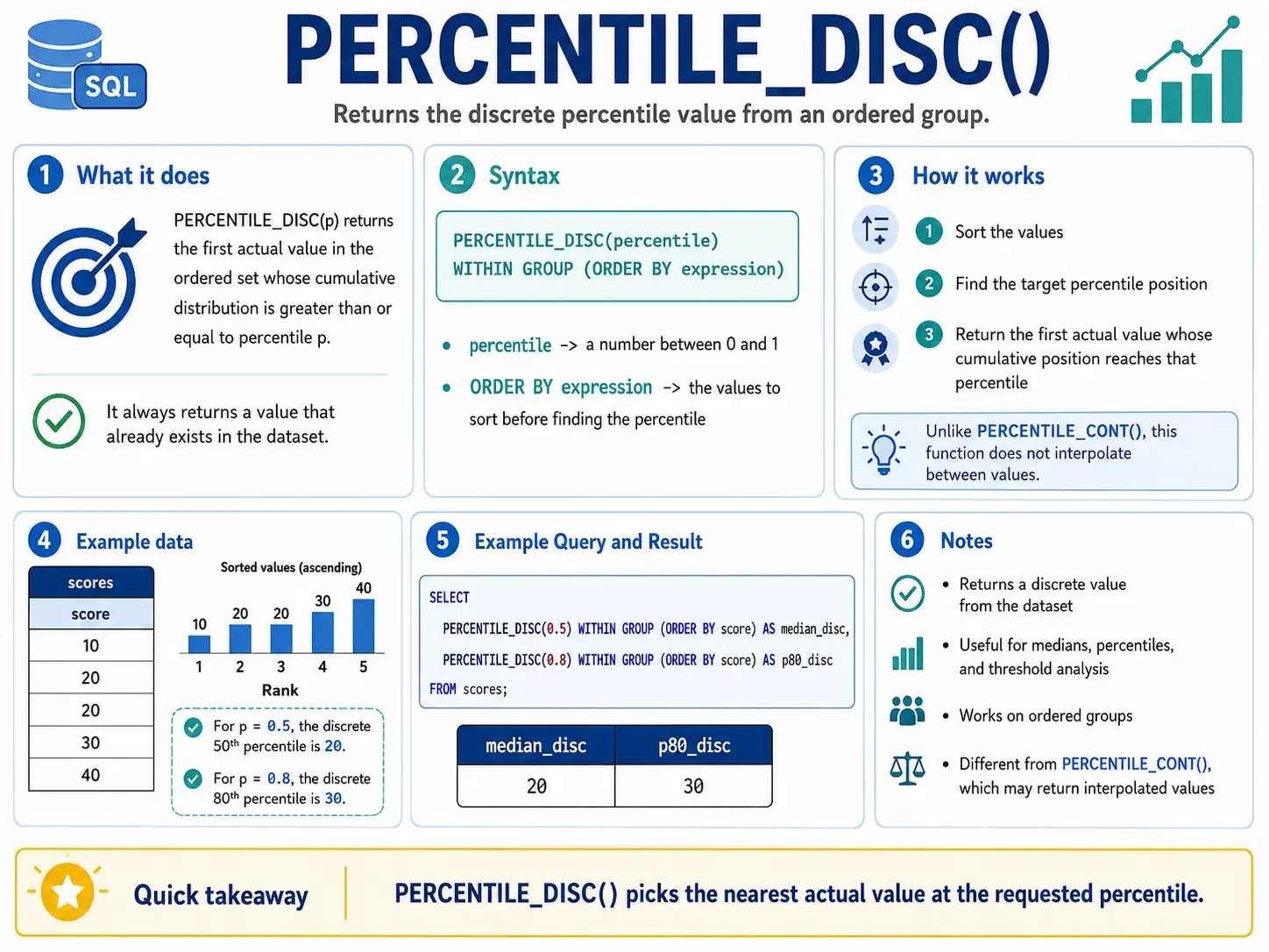
PERCENTILE_DISC(): Finding an Exact Percentile Value

PERCENTILE_DISC() helps you find a specific value from your data that represents a certain percentile (like the 50th percentile for the median). The key is that it will only return an actual value that exists in your data, it won’t invent a new one. It finds the first value whose cumulative distribution is greater than or equal to the percentile you ask for

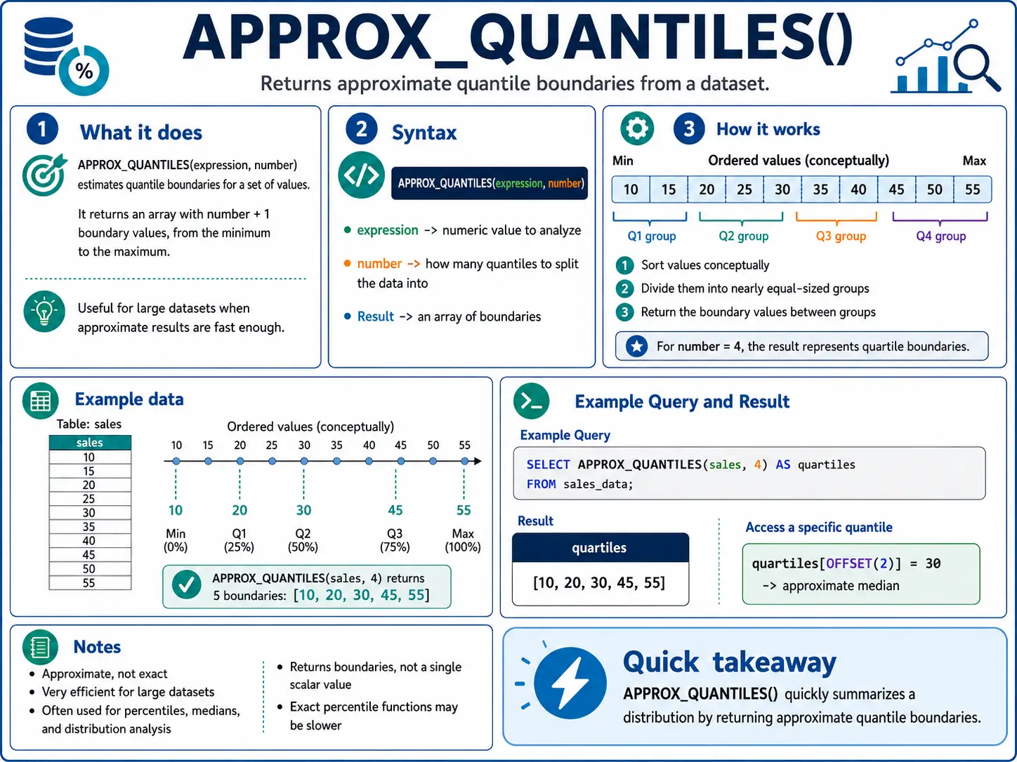
APPROX_QUANTILES(): (BigQuery) Fast Percentiles for Huge Data

When you have massive amounts of data, calculating exact percentiles can be very slow. APPROX_QUANTILES() gives you a very close estimate much faster. You tell it how many buckets you want (e.g., 100 for percentiles), and it returns an array of those approximate quantile values.

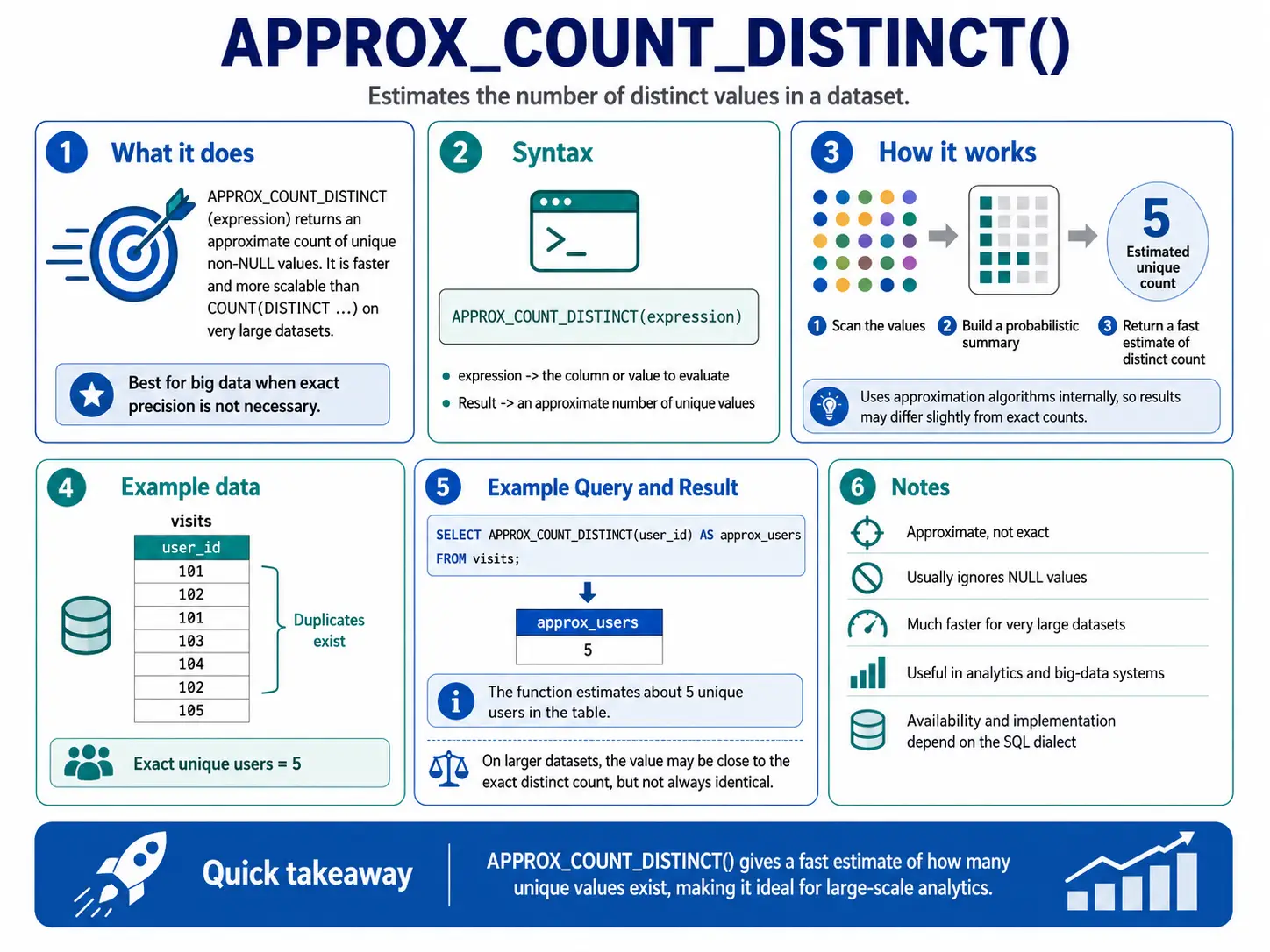
APPROX_COUNT_DISTINCT(): Fast Unique Counts

Similar to APPROX_QUANTILES(), this function gives you a fast estimate of how many unique items are in a huge dataset. It’s much quicker than COUNT(DISTINCT ...) when exactness isn’t critical, but speed is.

Aggregate Functions as Windows

You already know these functions (SUM, AVG, COUNT, MIN, MAX) from basic SQL. But when you add the OVER() clause, they become super powerful for calculating things like running totals and moving averages without squishing your data into single summary rows.

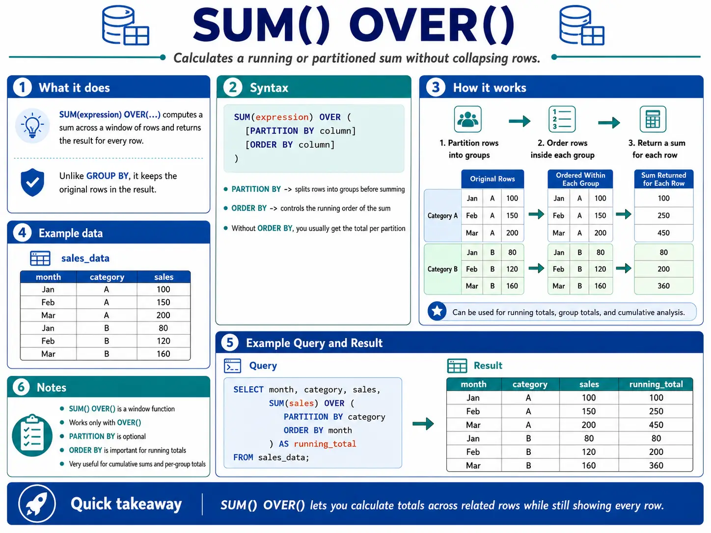
SUM() OVER(): The Running Total

SUM() with OVER() and an ORDER BY clause creates a running total. This means for each row, it adds up the current value and all the values before it in that group. It’s perfect for seeing how a total grows over time.

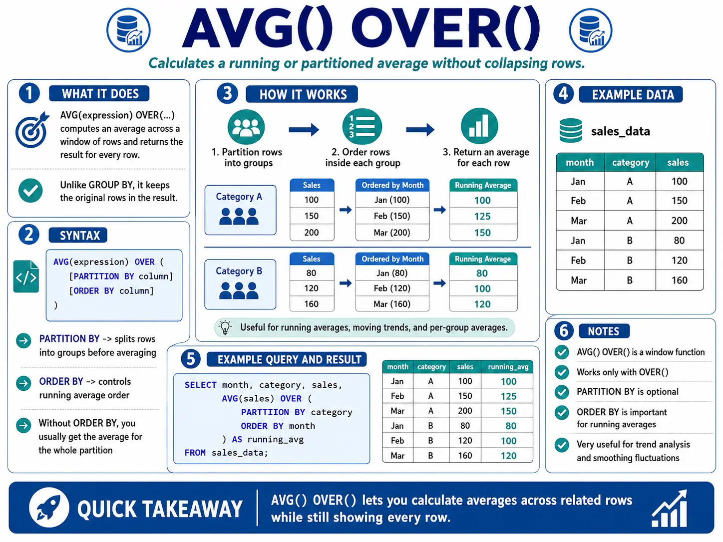
AVG() OVER(): The Moving Average

AVG() with OVER() and a specific window frame (like ROWS BETWEEN 6 PRECEDING AND CURRENT ROW) calculates a moving average. This is super useful for smoothing out data that jumps around a lot (like daily website visits) so you can see the real trends more clearly.

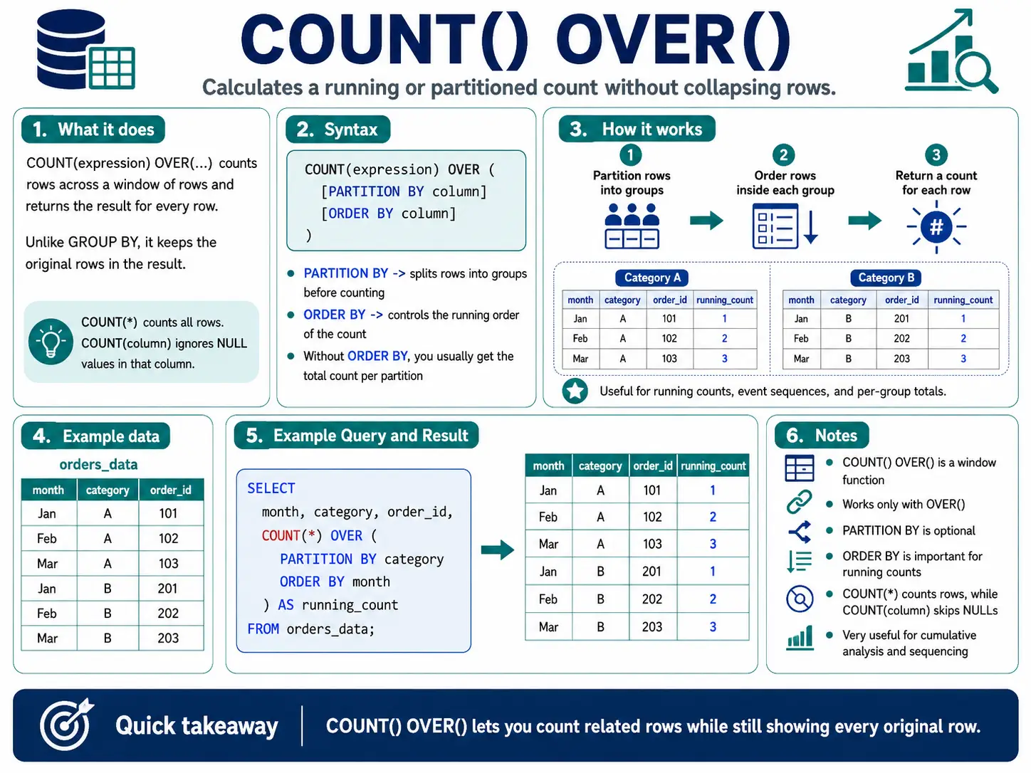
COUNT() OVER(): Counting Events in a Window

COUNT() with OVER() can give you a running count of events or count how many items fall within a specific window. This is useful for seeing how many times something has happened up to a certain point.

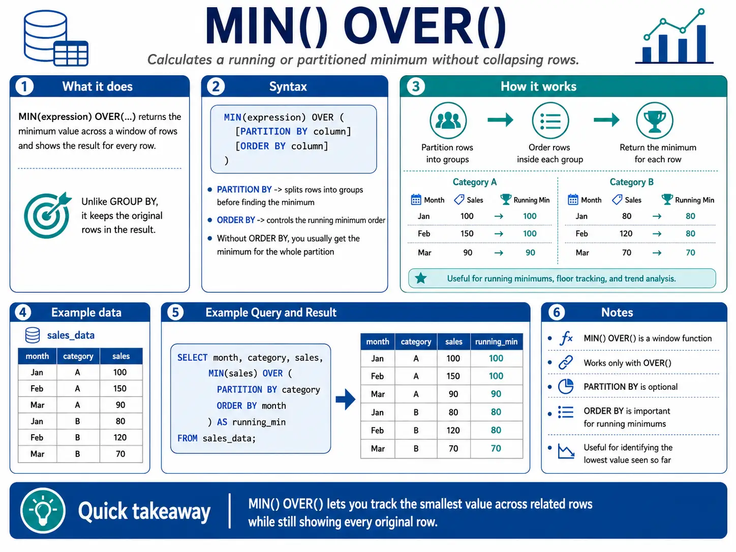
MIN() OVER(): Finding the Lowest Point in a Window

MIN() with OVER() helps you find the smallest value within a sliding window. This is useful for tracking minimums over a period, like the lowest stock price in the last month.

MAX() OVER(): Finding the Highest Point in a Window

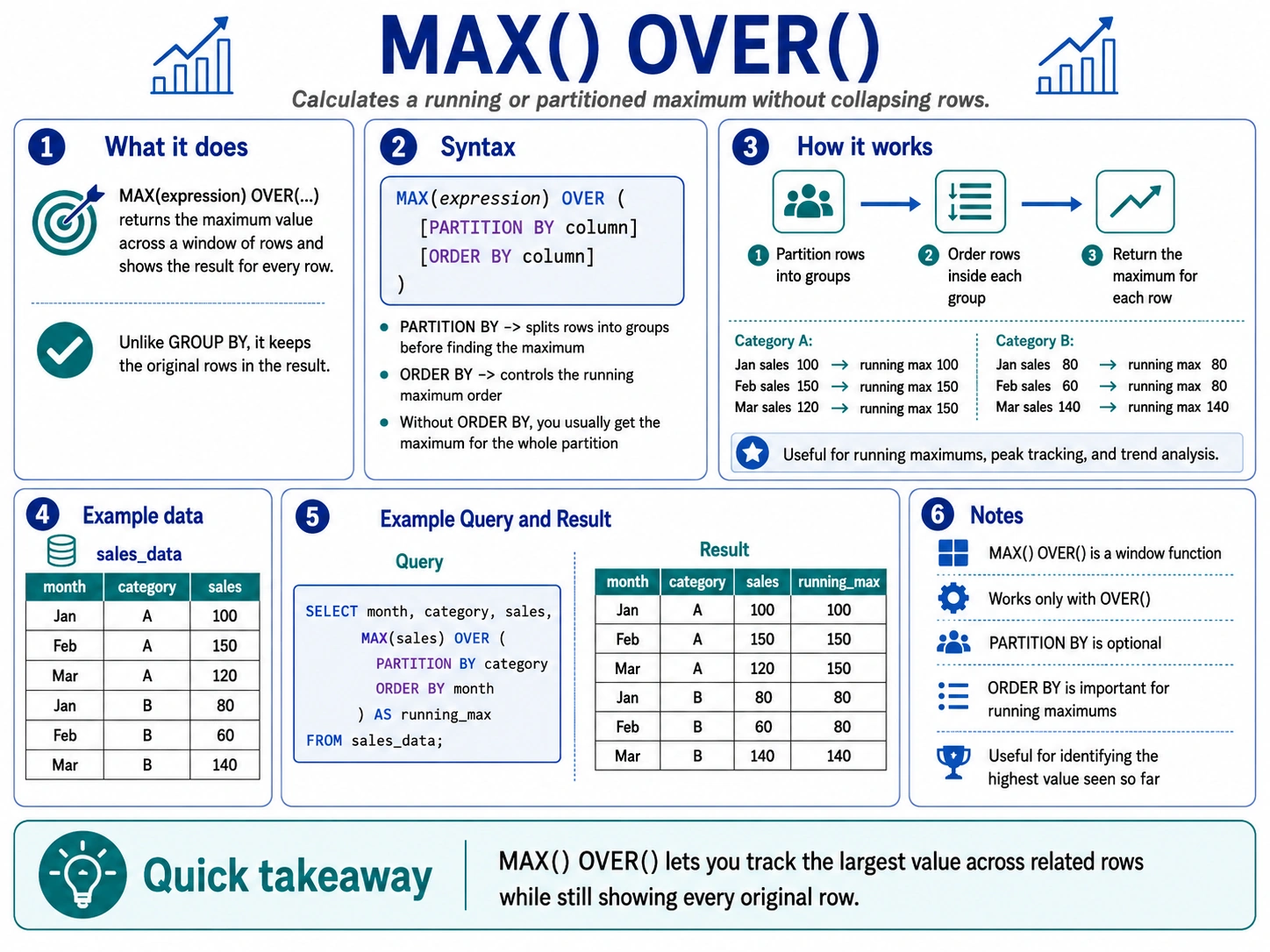
Similarly, MAX() with OVER() finds the largest value within a sliding window. This is great for tracking peaks, like the highest temperature recorded in the last 24 hours.

Specialized Analytic & Platforms Specific Functions

Beyond the common functions, many modern databases offer unique window functions that are super powerful for specific tasks. These might be a bit different depending on whether you’re using BigQuery, Snowflake, Oracle, or PostgreSQL, but they all help you do more advanced data science.

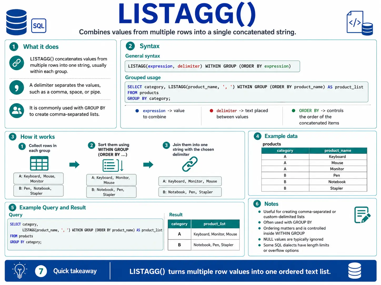
LISTAGG(): (Oracle/Snowflake) Collecting Text into One String

LISTAGG() takes values from many rows and squishes them into a single string, separated by something you choose (like a comma). It’s great for making lists of items related to a group.

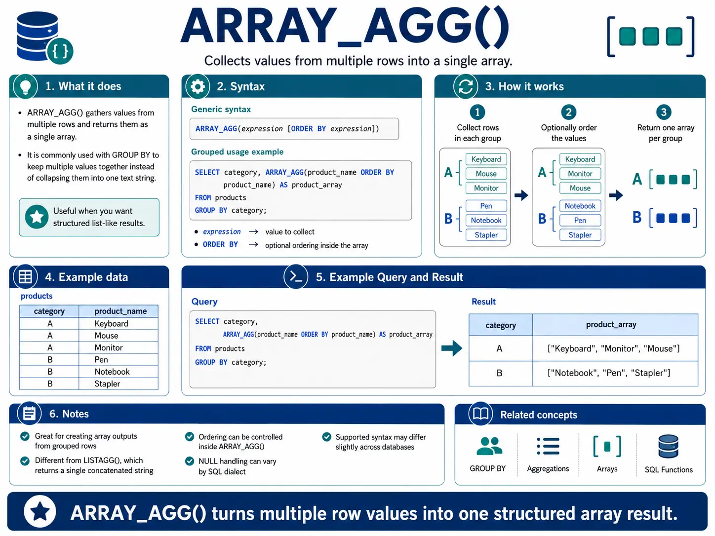
ARRAY_AGG(): (BigQuery/PostgreSQL) Gathering Items into a List (Array)

ARRAY_AGG() is similar to LISTAGG(), but instead of a single string, it collects values into an array (a structured list). This is very useful in databases that handle complex data types, letting you keep related items together.

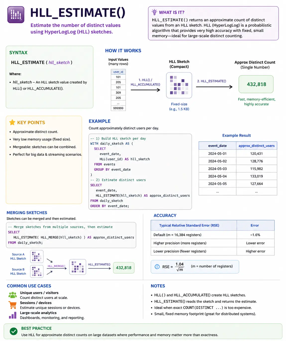
HLL_ESTIMATE(): (Snowflake) Quickly Counting Unique Things in Huge Data

HLL_ESTIMATE() uses a clever trick (called HyperLogLog) to quickly estimate how many unique items are in a very large dataset. When counting exact unique items is too slow, this function gives you a good-enough answer very fast.

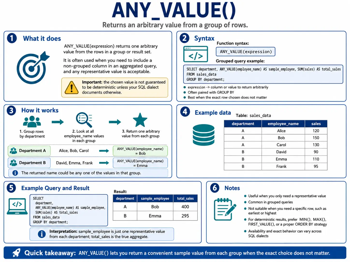
ANY_VALUE(): (BigQuery) Just Grab Any Value

ANY_VALUE() is a simple function that returns any value from a group. It’s useful when you don’t care which specific value you get, just that you get one from that group. This helps avoid errors when you need to include a non-grouped column in your results.

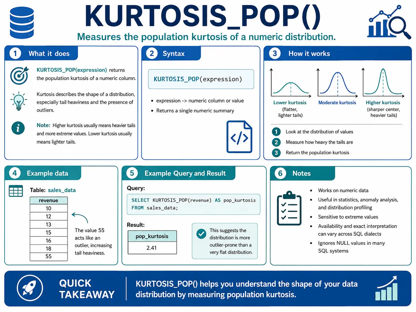
KURTOSIS_POP(): (Oracle) How “Peaky” or “Flat” is My Data?

KURTOSIS_POP() measures the “tailedness” of your data distribution. In simple terms, it tells you if your data has very few extreme values (flat) or many extreme values (peaky). This is important for understanding risk or unusual events.

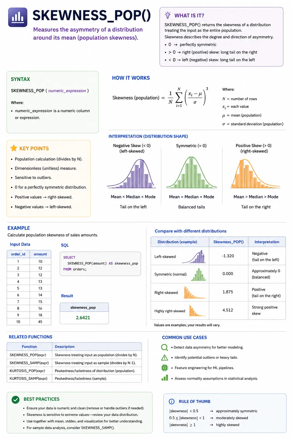
SKEWNESS_POP()

SKEWNESS_POP() measures how symmetrical your data is. If your data is perfectly balanced around its average, it has zero skewness. Positive skew means more data is on the left (a long tail to the right), and negative skew means more data is on the right (a long tail to the left).

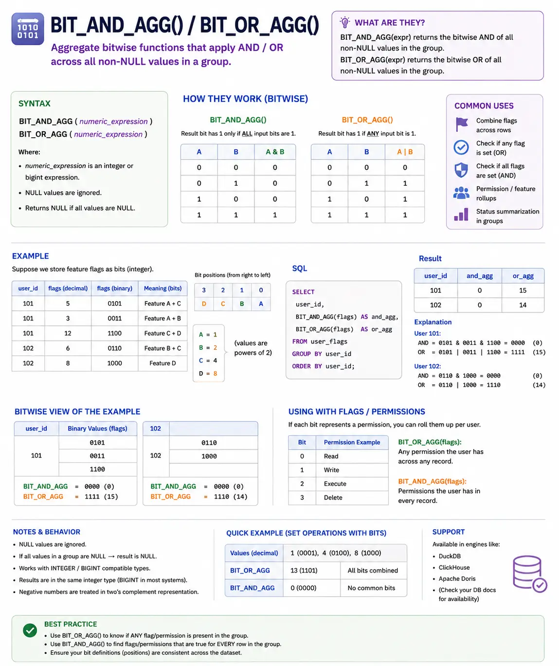
BIT_AND_AGG() / BIT_OR_AGG(): (BigQuery/Oracle) Combining Binary Flags

These are special functions for working with binary numbers (bits). If you have flags or permissions stored as bits, BIT_AND_AGG() will find the common bits (permissions) across a group, and BIT_OR_AGG() will find all bits (permissions) present in at least one item in the group.

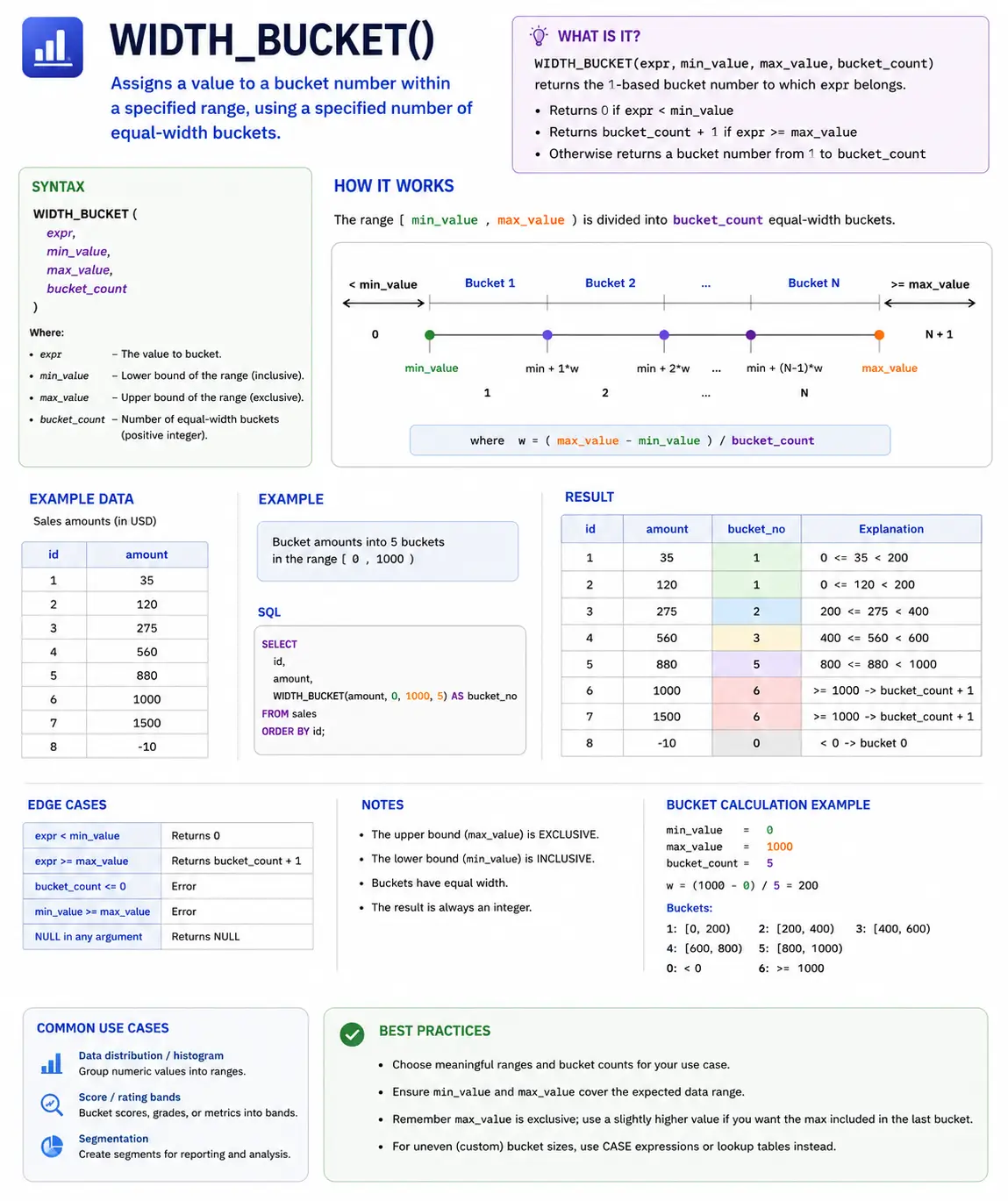
WIDTH_BUCKET(): Grouping Data into Buckets

WIDTH_BUCKET() is a useful function for dividing a range of values into a specified number of equally sized buckets or bins. This is great for creating histograms or categorizing continuous data.

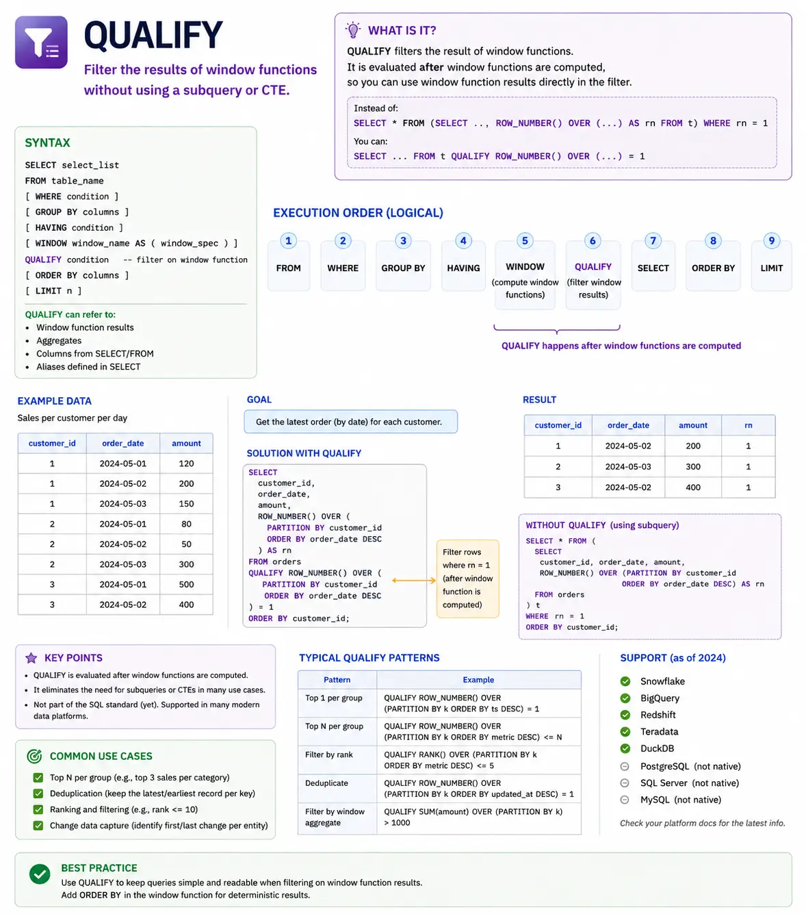
QUALIFY: Filtering Window Function Results (Snowflake/BigQuery)

QUALIFY is not a function itself, but a powerful clause available in some modern SQL dialects (like Snowflake and BigQuery) that lets you filter the results of window functions directly, without needing to wrap your query in a subquery or CTE. It makes your code much cleaner when you want to select rows based on a window function’s output.

Understanding SQL’s Execution Order: When Do WIndow Functions Run?

To use window functions effectively, you need to understand when SQL actually calculates them. SQL doesn’t read your query from top to bottom. It follows a specific logical order:

1. FROM & JOIN: First, SQL gets the tables and joins them together.
2. WHERE: Then, it filters out rows that don’t match your conditions.
3. GROUP BY: Next, it groups rows together for regular aggregate functions.
4. HAVING: It filters those grouped rows.
5. SELECT: Now, it picks the columns you asked for. This is where Window Functions are calculated!
6. DISTINCT: It removes duplicate rows.
7. ORDER BY: Finally, it sorts the final results.
8. LIMIT / OFFSET: It restricts the number of rows returned.

Why does this matter? Because window functions are calculated in step 5 (SELECT), they happen after the WHERE clause. This means you cannot use a window function directly in a WHERE clause to filter your results.

Conclusion

SQL Window Functions are an absolute must-have skill for any data scientist. They allow you to perform complex, row-level calculations without losing the detail of your original data. By mastering these 40 functions from basic ranking to advanced statistical analysis you’ll be able to write cleaner, more efficient queries and uncover deeper insights from your datasets.

Frequently Asked Questions