Iloc vs Loc in Pandas: A Guide with Examples 

Pandas DataFrames provide powerful tools for selecting and indexing data efficiently. The two most commonly used indexers are .loc and .iloc. The .loc method selects data using labels such as row and column names, while .iloc works with integer positions based on a 0-based index. Although they may seem similar, they function differently and can confuse beginners.

In this guide, you’ll learn the key differences between .loc and .iloc through practical examples. Using a real dataset, we’ll show how each method works and what kind of output they produce in real use cases.

Understanding .loc and .iloc in Pandas DataFrames

The Pandas library provides DataFrame objects with two attributes .loc and .iloc which users can employ to extract specific data from their DataFrame. These two functions display identical syntax through their implementation of indexers whereas they show different behavior when processing indexers. The .loc function treats its input as row or column label names while the .iloc function treats its input as numeric row or column indexes. The two functions allow users to filter data through the use of boolean arrays. 

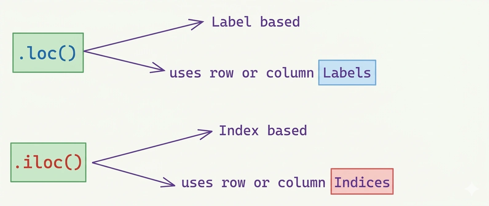
• .loc: Label-based indexing. Use actual row/column labels or boolean masks (aligned by index) 
• .iloc: Integer position-based indexing. Use numeric indices (0 to N-1) or boolean masks (by position). 

For Example:  

Let’s assume your training data covers information until October of the year 2025. Therefore, the date index allows .loc['2025-01-01':'2025-01-31'] to perform label-based slicing which .iloc requires through date conversion to integer positions for its function. The function of .loc should be selected when handling label data while .iloc should be used when working with numerical data that represents positions. 

import pandas as pd 
import numpy as np 

dates = pd.date_range(start="2025-01-01", periods=40) 

df = pd.DataFrame({ 
   "value": np.arange(40) 
}, index=dates) 

df.loc["2025-01-01":"2025-01-31"][:2]

	value
2025-01-01	0
2025-01-02	1

df.iloc[0:2] 

	value
2025-01-01	0
2025-01-02	1

Working with .loc: Label-Based Indexing in Practice 

Before jumping into the hands-on part lets create a dataset first. 

import pandas as pd 

# Sample DataFrame 
df= pd.DataFrame({ 

   "Name": ["Alice Brown", "Lukas Schmidt", "Ravi Kumar", "Sofia Lopez", "Chen Wei"], 
   "Country": ["Canada", "Germany", "India", "Spain", "China"], 
   "Region": ["North America", "Europe", "Asia", "Europe", "Asia"], 
   "Age": [30, 45, 28, 35, 50] 
}, index=["C123", "C234", "C345", "C456", "C567"]) 

df

The DataFrame df contains index labels which range from C123 to C567. We will use .loc to select subsets of this data through label-based selection. 

	Name	Country	Region	Age
C123	Alice Brown	Canada	North America	30
C234	Lukas Schmidt	Germany	Europe	45
C345	Ravi Kumar	India	Asia	28
C456	Sofia Lopez	Spain	Europe	35
C567	Chen Wei	China	Asia	50

Accessing a Single Row with .loc 

The user can obtain a single row by its label through passing the label to .loc as the row indexer. The result is a Series of that row: 

row = df.loc["C345"] 

row 

Name              Ravi Kumar 
Country              India 
Region                Asia 
Age                     28 
Name: C345, dtype: object

The function df.loc[“C345”] retrieves the data from the row which has index value ‘C345’. The data includes all columns in the dataset. The system uses label-based access, so attempting to access df.loc[“C999”] (a non-existent entry) will result in a KeyError. 

Retrieving Multiple Rows with .loc 

To select multiple non-consecutive rows requires us to provide their respective row labels through the row_indexer function. The operation requires us to use two sets of square brackets because we need one set for .loc standard operations and another set for the label list. 

The line df.loc[['row_label_1', 'row_label_2']] will return the two rows of the df DataFrame specified in the list. Let’s say we wanted to know not only the information on Ali Khan but as well on David Lee: 

subset = df.loc[["C345", "C567"]] 

subset

	Name	Country	Region	Age
C345	Ravi Kumar	India	Asia	28
C567	Chen Wei	China	Asia	50

Slicing Rows Using .loc 

We can select a range of rows by passing the first and last row labels with a colon in between: df.loc[‘row_label_start’:’row_label_end’]. The first four rows of our DataFrame can be displayed with this method: 

slice_df = df.loc["C234":"C456"] 

slice_df

	Name	Country	Region	Age
C234	Lukas Schmidt	Germany	Europe	45
C345	Ravi Kumar	India	Asia	28
C456	Sofia Lopez	Spain	Europe	35

The df.loc["C234":"C456"] function returns the range of rows from ‘C234’ to ‘C456’ which includes ‘C456’ (unlike normal Python slicing).The .loc method will select all records within a .loc range that includes both starting point and ending point when your DataFrame index is sorted. 

Filtering Rows Conditionally with .loc 

We can also return rows based on a conditional expression. The system will display matching rows when we apply a specific condition to filter all available data. The corresponding syntax is df.loc[conditional_expression], with the conditional_expression being a statement about the allowed values in a specific column. 

The statement can only use the equal or unequal operator for non-numeric columns such as Name and Country because these fields do not have any value hierarchy. We could, for instance, return all rows of where age >30: 

filtered = df.loc[df["Age"] > 30] 

filtered

	Name	Country	Region	Age
C234	Lukas Schmidt	Germany	Europe	45
C456	Sofia Lopez	Spain	Europe	35
C567	Chen Wei	China	Asia	50

The expression df["Age"] > 30 generates a boolean Series which uses the same indices as df. The boolean Series gets passed to .loc[...] which extracts rows that match the condition which returns all rows where the condition is True. The .loc function uses the DataFrame index to create correct subsets which eliminates the need for specific numeric position details. 

Selecting a Single Column via .loc 

The selection of columns needs us to provide the column_indexer argument which follows after we define our row_indexer argument. When we want to use only our column_indexer we must indicate our intention to select all rows while applying column filters. Let’s see how we can do it! 

A user can select an individual column through the column_indexer when they provide the column label. The process of retrieving all rows requires us to use row_indexer with a basic colon symbol. We arrive at a syntax that looks like this: df.loc[:, 'column_name']. 

The display of country’s names will take place in the following manner: 

country_col = df.loc[:, "Country"] 

country_col

C123     Canada 
C234    Germany 
C345      India 
C456      Spain 
C567      Chin
Name: Country, dtype: str

Here, df.loc[:, "Country"] means “all rows (:) and the column labeled ‘Country’”. This returns a Series of that column. Note that the row index is still the customer IDs. 

Extracting Multiple Columns with .loc 

The process of choosing multiple rows requires us to provide a list with column names which we use to retrieve nonsequential DataFrame columns through the command df.loc[:, [col_label_1, 'col_label_2']]. 

The process of adding Name and Age to our most recent result requires the following method. 

name_age = df.loc[:, ["Name", "Age"]] 

name_age

	Name	Age
C123	Alice Brown	30
C234	Lukas Schmidt	45
C345	Ravi Kumar	28
C456	Sofia Lopez	35
C567	Chen Wei	50

Column Slicing Using .loc 

country_region = df.loc[:, "Country":"Region"] 

country_region

	Country	Region
C123	Canada	North America
C234	Germany	Europe
C345	India	Asia
C456	Spain	Europe
C567	China	Asia

Selecting Rows and Columns Together Using .loc 

The system allows users to define both row_indexer and column_indexer parameters. This method enables users to extract specific data from the DataFrame by selecting one cell. The command df.loc['row_label', 'column_name'] allows us to select one specific row and one specific column from the data set.  

The below example shows how to retrieve customer data which includes their Name and Country and Region information for customers who are older than 30 years. 

df.loc[df['Age'] > 30, 'Name':'Region'] 

	Name	Country	Region
C234	Lukas Schmidt	Germany	Europe
C456	Sofia Lopez	Spain	Europe
C567	Chen Wei	China	Asia

Using .iloc: Integer-Based Indexing Explained 

The .iloc indexer functions like .loc indexer but it operates through numeric index values. The system only utilizes numeric indexes because it does not consider any row or column identifiers. You can use this function to select items through their physical location or when your naming system proves difficult to use. The two systems differ mainly through their slicing methods because .iloc uses standard Python slicing which excludes the stop index. 

Accessing a Single Row with .iloc 

You can select one specific row by using its corresponding integer index which serves as the row_indexer. We don’t need quotation marks since we are entering an integer number and not a label string as we did with .loc. The first row of the DataFrame named df can be accessed through the command df.iloc[2]. 

row2 = df.iloc[2] 

row2

Name       Ravi Kumar 
Country         India 
Region           Asia 
Age                28 
Name: C345, dtype: object

The third row of the data set appears as a Series which can be accessed through df.iloc[2]. The data in this section exactly matches the data in df.loc["C345"] because ‘C345’ is at position 2. The integer 2 functioned here as our method of accessing the data instead of using the label ‘C345’. 

Retrieving Multiple Rows with .iloc 

The .iloc method allows users to select multiple rows through the same process used by .loc, which requires us to input row indexes as integers contained within a list that uses squared brackets. The syntax looks like this: df.iloc[[2, 4]]. 

The respective output in our customer table can be seen below: 

subset_iloc = df.iloc[[2, 4]] 

subset_iloc

	Name	Country	Region	Age
C345	Ravi Kumar	India	Asia	28
C567	Chen Wei	China	Asia	50

The command df.iloc[[2, 4]] retrieves the third and fifth rows from the data. The output shows their labels for clarity, but we chose them by position. 

Slicing Rows Using .iloc 

The selection of row slices requires us to use a colon between two specified row index integers. Now, we have to pay attention to the exclusivity mentioned earlier.  

slice_iloc = df.iloc[1:4] 

slice_iloc

	Name	Country	Region	Age
C234	Lukas Schmidt	Germany	Europe	45
C345	Ravi Kumar	India	Asia	28
C456	Sofia Lopez	Spain	Europe	35

The line df.iloc[1:4] serves as a demonstration for this particular principle. The slice begins at index number 1 which represents the second row of the table. The index integer 4 represents the fifth row, but since .iloc is not inclusive for slice selection, our output will include all rows up until the last before this one. The output will show the second row together with the third row and the fourth row of data. 

Selecting a Single Column via .iloc 

The logic of selecting columns using .iloc follows what we have learned so far. The system operates through three different methods which include single column retrieval and multiple column selection and column slice operations. 

Just like with .loc, it is important to specify the row_indexer before we can proceed to the column_indexer. The code df.iloc[:, 2] allows us to access all rows of the third column in df. 

region_col = df.iloc[:, 2] 

region_col

C123    North America 
C234           Europe 
C345             Asia 
C456           Europe 
C567             Asia 
Name: Region, dtype: str

Extracting Multiple Columns with .iloc 

To select multiple columns that are not necessarily subsequent, we can again enter a list containing integers as the column_indexer. The line df.iloc[:, [0, 3]] returns both the first and fourth columns. 

name_age2 = df.iloc[:, [0, 3]] 

name_age2

	Name	Age
C123	Alice Brown	30
C234	Lukas Schmidt	45
C345	Ravi Kumar	28
C456	Sofia Lopez	35
C567	Chen Wei	50

The command df.iloc[:, [0, 3]] retrieves columns 1 and 4 which are located at positions 0 and 3 named “Name” and “Age”. 

Column Slicing Using .iloc 

The .iloc slicing method uses column_indexer logic which follows the same pattern as row_indexer logic. The output excludes the column which corresponds to the integer that appears after the colon. To retrieve the second and third columns, the code line should look like this: df.iloc[:, 1:3]. 

country_region2 = df.iloc[:, 1:3] 

country_region2

The df.iloc[:, 1:3] function retrieves the columns from the first two positions, which include “Country” and “Region” while excluding the third position. 

	Country	Region
C123	Canada	North America
C234	Germany	Europe
C345	India	Asia
C456	Spain	Europe
C567	China	Asia

Selecting Rows and Columns Together Using .iloc 

The .loc method enables us to choose indexers through list notation with square brackets or through slice notation with colon. The .iloc method enables users to select rows through conditional expressions however this method is not advisable. The .loc method combined with label names offers users an intuitive method which decreases their chances of making mistakes. 

subset_iloc2 = df.iloc[1:4, [0, 3]] 

subset_iloc2

The code df.iloc[1:4, [0, 3]] selects from the DataFrame all rows between positions 1 and 3 which excludes position 4 and all columns at positions 0 and 3. The result is a DataFrame of those entries. 

	Name	Age
C234	Lukas Schmidt	45
C345	Ravi Kumar	28
C456	Sofia Lopez	35

.iloc vs .loc: Choosing the Right Indexing Method 

The choice between .loc and .iloc depends on the specific situation. Like what kind of problem we are trying to solve while dealing with the data. 

• Using the .loc function provides access to data through its corresponding labels. The .loc function allows direct access to labels when your DataFrame index includes meaningful labels which contain dates and IDs and names.  
• Using the .iloc function enables users to access data according to its specific position. The .iloc function becomes easy to use when users need to loop through numeric values or already know their specific positions.  
• Slicing preference: If you want inclusive slices and your index is sorted, .loc slices include the end label. The .iloc function provides predictable results for users who want to apply the standard Python slicing method which excludes the final element. 
• Performance: The two methods present equal speed capabilities since performance depends on the task. In most situations, you should select the option that corresponds with your intended use which involves either labels or positions without needing to perform extra transformation. 
• Practical guidelines: The guidelines for using DataFrames with labeled indexes and named columns show that .loc performs better in terms of readability. The function .iloc becomes more beneficial during code development which requires you to observe your progress by counting active rows. 

Common Mistakes with .loc and .iloc 

Sometimes the functions .loc and .iloc create error problems which require careful handling. The most frequent errors arise from these situations: 

• KeyError with .loc: When you use .loc with a nonexistent label, it raises a KeyError. The code df.loc["X"] will generate a KeyError because “X” does not exist in the index. You need to verify that the label has been entered correctly. 
• IndexError with .iloc: Pandas IndexError occurs when you request a row or column through .iloc which exceeds the valid row limit. You should verify the boundaries before cutting data at specific positions. 
• Inclusive vs Exclusive slices: The inclusive slice behavior of df.loc[a:b] which includes element b contrasts with the exclusive slice behavior of df.iloc[a:b] which excludes element b. This often leads to off-by-one issues. 
• Mixing up label and position: Label and position exist as distinct elements which you should keep separate. The system treats index labels 0,1 and 2 as numeric values which means df.loc[0] accesses the index label 0 instead of the first row. The system treats df.iloc[0] as a command which always selects the first row of data irrespective of its assigned label. 
• Using ix (deprecated): The ix function has been eliminated from Pandas because it presented an outdated implementation which combined two different functions into one. You should use .loc or .iloc exclusively. 
• Chain indexing: The method df[df.A > 0].B = .... needs to be replaced with .loc which will enable you to filter data and execute assignment operations while preventing unexpected “SettingWithCopy” errors from occurring.  

Conclusion 

Pandas offers two key tools for DataFrame subsetting: .loc and .iloc. The .loc method uses labels (row/column names), while .iloc relies on integer positions. A key difference is slicing: .loc includes the end label, whereas .iloc follows Python’s exclusive slicing. Mastering both helps you select data efficiently, apply filters, and write cleaner, more reliable data manipulation code.

Frequently Asked Questions