This article was published as a part of the Data Science Blogathon.
Introduction
In the time series prediction, it is common to use the historical value of the target variable to predict its future value. If the target variable depends on multiple attributes and each attribute forms a time series prediction, how could we make use of these attributes to predict the future value?
For example, RSI is a good indicator to determine the direction of the trend of the stock price. In my other article, I tried to use the RSI as the Machine Learning (ML) feature to predict the stock price return. What if we have multiple indicators? In this article, I will use multiple stock market indicators to demonstrate how to use multiple ML features in the Time Series Prediction. Hyper-parameter tuning will also be explained. I will evaluate the result from the perspective of the trading strategy at the end.
Complete code can be found in my notebook.
I would choose these 3 indicators as the ML features: (1) RSI, (2) MACD, and (3) Bollinger Bands.
Chosen Indicators
1. RSI – Relative Strength (RS) and Relative Strength Indicator (RSI) can be computed from the Moving Average (MA) of the historical positive price difference (%) divided by that of the negative price difference (%).
RS = (MA of positive difference) / (MA of negative difference)
RSI = 100–100/(1+RS)
Oscillator of RSI = current RSI value – MA of RSI
We will use the Oscillator of the RSI as one of the ML features.
OsRSI(i,j) = (i-day RSI) – (j-day-MA of i-day-RSI)
2. MACD – Moving Average Convergence Divergence (MACD) can be calculated from the subtraction of the exponential moving average (EMA) between 12 days and 26 days.
MACD = (12-day EMA) – (26-day EMA)
For simplicity, I use the simple moving average (MA) instead of EMA so that there is no need to tune the smoothing factor of EMA.
SimpMACD(i,j) = (i-day-MA) – (j-day-MA)
3. Bollinger Bands – Bollinger Bands consists of 2 lines based on the normal distribution of the last i-days.
Upper Band = MA + 2 * (standard deviation)
Lower Band = MA – 2 * (standard deviation)
The current MA will be compared with the above 2 bands to indicate whether it is an upward trend or a downward trend.
Upper Band Indicator: UpBB(i,j) = (i-day-MA) – (j-day-Upper Band)
Lower Band Indicator: LowBB(i,j) = (i-day-MA) – (j-day-Lower Band)
Feature Engineering
All the above indicators have the time scope in the calculation of the Moving Average (MA). In contrast to the manual analysis, we do not need to fix the value of the time scope because we can loop the time scope over a reasonable range of values.
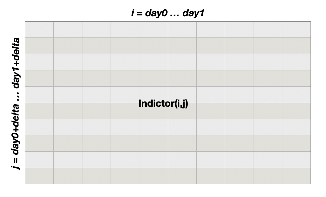
For each indicator, I form a matrix by looping the indicator over “i” and “j” as the number of rows and columns, where the index (“i”) is ranging from day0 to day1 days, and j = I + delta.
ML Model
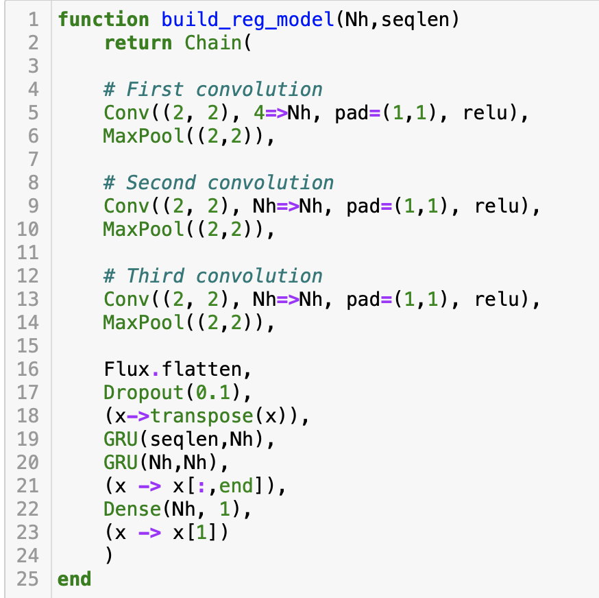
Similar to my other article, the above feature Matrix can be fed into the Convolution Neural Network (CNN) for pattern recognition. Each feature Matrix would be fed as the channel of the CNN layer. As there are 4 features, the channel input of the CNN is 4. I also use the Matrix of the current day and the previous (“SEQLEN”-1) days to form a sequence of Matrix as the fourth dimension input of the CNN layer. The output of the Convolution will be flattened and then be fed to the layer of GRU, and finally to a linear layer to predict the rate of return of the next day.
Below is the code of the model, which is written in Julia, with the ML package Flux.
Shape matching
In coding multiple neural network layers, matching the input shape and the output shape of each layer is critical.
The convolution layer (Conv) input requires a 4-dimension tensor.
- The first 2 dimensions are the size of the input image. As we use the feature matrix as the input, the shape of the matrix becomes the size of the image as the first two dimension input. That is day1 – day0.
- The third dimension of the CNN input is the number of channels, where each indicator feature is 1 channel, so the number of channels of the CNN would be 4.
- The fourth dimension of the CNN input would be the time step of the feature matrix with its historical values, so it would be SEQLEN.
Match the CNN output with the GRU input:
- The output of the CNN layers will be flattened by the function flatten, which will compress the output into a 2D tensor by fixing the last dimension (SEQLEN).
- To connect the output to the GRU layer, it has to match the last dimension (SEQLEN) with the GRU hidden state by transposing the tensor.
- As the prediction is just a 1-time step in the next day, the last tensor of the GRU output is selected.
Finally, the GRU output will be fed into the linear layer (Dense layer) to get the prediction.
Training Convergent
To make the ML training convergent, I used the 5-day moving average of the rate of return of the close price as the target variable. It is because a moving average can smoothen the fluctuation of the price change.
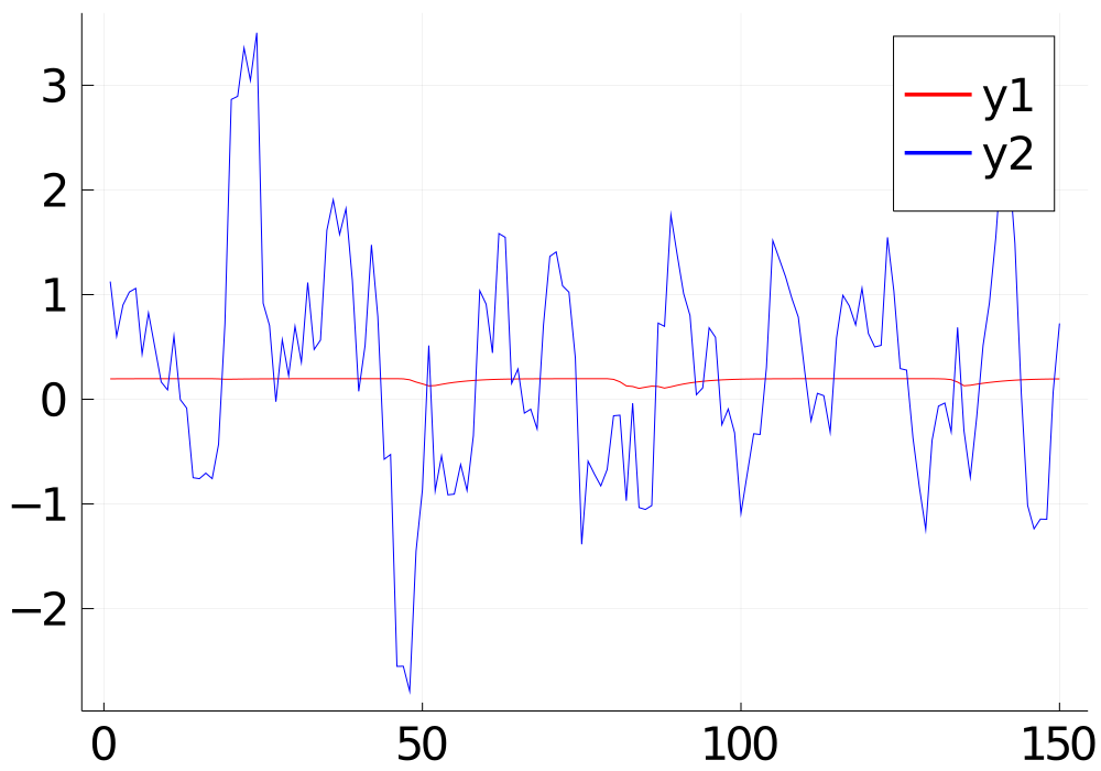
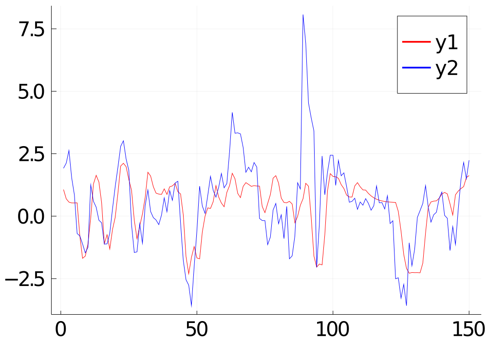
Choosing the right value for the learning rate is also important, otherwise, the training would not be convergent. Other parameters such as the time range of the indicators, the sequence length, and the number of the hidden state may also affect the convergence. If the training cannot converge, the prediction will be just a flat line, as shown in the red line in the graph below. Suitable values for these parameters can be found by using hyper-parameter tuning.
Hyper-parameter tuning
In Julia, hyper-parameter tuning can be easily done by the package “Hyperopt“, by just a few lines of code below.
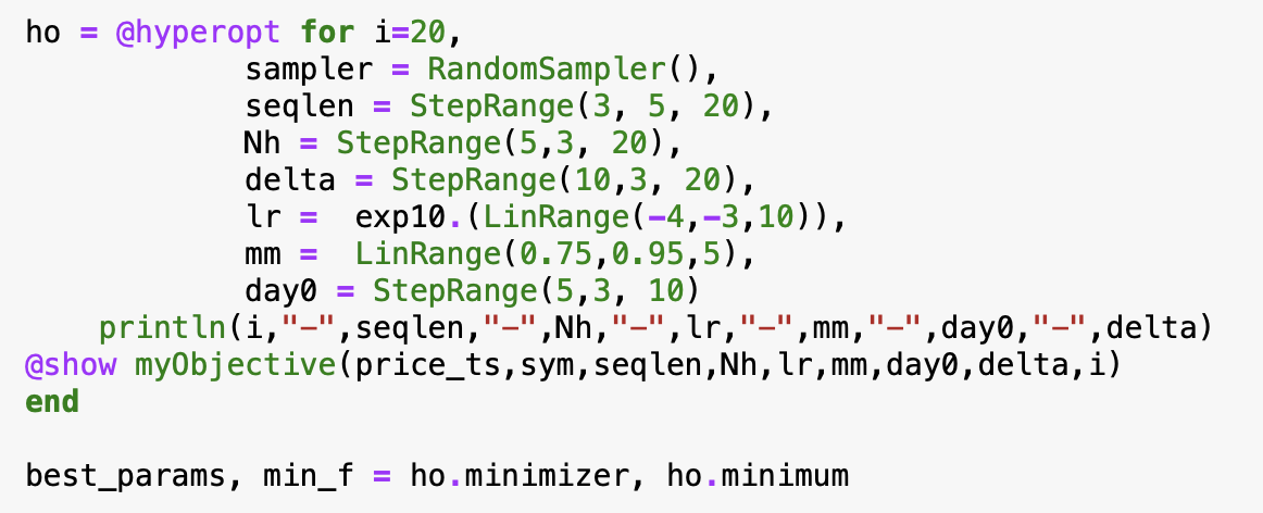
First, define the range of each parameter for the tuning:
- The learning rate (LR) and the momentum (MM) of the RMSProp.
- The number of hidden state (Nh) of the CNN and GRU
- The sequence length of the time step (SEQLEN)
- The time scope of the indicator matrix (day0, and day0+delta)
- day1 = day0 + delta – 1
Hyperopt would loop over the range of the above parameters randomly and then find out the minimum of the objective cost, which is the value returned by the objective function (“MyObective”). The objective function performs the model training with the specified parameters and returns the validation loss as the objective cost.
From the perspective of trading, predicting the up/down trend correctly is more important, so I adjusted the object cost by the prediction accuracy in the hyper-parameter optimization.
Result
For each round of training, I held out the last 150 data points as the unseen testing data.
The graph below is the predicted value (red line) and the actual value of the testing data (blue line) after the hyper-parameter tuning. The prediction fits quite well with the actual value. The MSE of the testing is 0.66. From the perspective of predicting the up/down correctly, the accuracy is 0.73.
Below are the final values of the hyper-parameters:
|
|
|
|
|
|
|
|
|
|
|
|
|
|
Trading Strategy
The simplest trading strategy can be the following: The positive predicted value will be the buy-signal, and the negative will be the sell-signal. However, since the rate of return is calculated by the closing price when today’s closing price is used to calculate the rate of return as the input of the model, the market had already been closed and no trade order could be placed. For practical reasons, we can only use the price 5 minutes before the market close to approximate today’s close price, so that we still have time to place an order according to the model prediction.
Back-testing
I use the testing data to compute the model prediction and then map it to the position of 1 or 0. For those days of position 1, I add up the rate of return of the close price. The total return gained in the testing period (150 days) is 38%. Whether it is good or bad? Let’s compare with the baseline. I add up all the rates of return of the testing period. The baseline return gained is 45%. Oh! that means the model prediction cannot do any good. Why?
One of the main reasons is that the target variable of the model is the 5-day moving average (MA) for the sake of the training convergence. However, the MA of the next day being positive does not mean the rate of return for the next day being positive. During my investigation, if I compare the predicted value against the daily rate of return instead of the MA of the rate of return, the accuracy dropped from 73% to 52%.
If I can find a way to estimate the daily rate of return based on the MA, I may get a better result.
The media shown in this article are not owned by Analytics Vidhya and is used at the Author’s discretion.


%202.jpg)
How is your model performing for post covid period? Especially if model training was done for pre-covid period and prediction needs to be done for longish term post pandemic? If the answer is is not doing too well, what are your suggestions to get better at it?
Hi, nice article. I'm also interested in developing trading strategy using ML. Have you considered LSTM? I read that it is the go-to model for time series. Also, why did you choose CNN? I thought it is best for image data.