This article was published as a part of the Data Science Blogathon.
Introduction on Bayesian Approach
The entire world of statistical rigour is split into two parts one is a Bayesian approach and the other is a frequentist. And it has been a moot point for statisticians throughout the century which one is better than the other. It is safe to say that the century has been dominated by frequentist statistics. Many algorithms that we use now namely least square regression, and logistic regression are a part of the frequentist approach to statistics. Where the parameters are always constant and predictor variables are random. While in a Bayesian world the predictors are treated as constants while the parameter estimates are random and each of them follows a distribution with some mean and variance. It gives us an extra layer of interpretability as the output is not any more a single point estimate but rather a distribution. This fundamentally separates Bayesian statistical inference from frequentist inference for statistical analysis. But there is a big trade-off as nothing comes free in this vain world which is one of the major reasons for its limited practical use.
So, in this article, we are going to explore the Bayesian method of regression analysis and see how it compares and contrasts with our good old Ordinary Least Square (OLS) regression. So, before delving into Bayesian rigour let’s have a brief primer on frequentist Least Square Regression.
Ordinary Least Square (OLS) Regression
This is the most basic and most popular form of linear regression that you are already accustomed to and yes this uses a frequentist approach for parameter estimation. The model assumes the predictor variables are random samples and with a linear combination of them we finally predict the response variable as a single point estimate. And to account for random sampling we have a residual term that explains the unexplained variance of the model. And this residual term follows a normal distribution with a mean of 0 and a standard deviation of sigma. The hypothesis equation for OLS is given by,
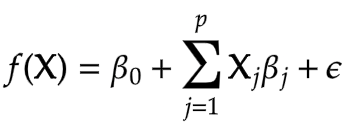
Here the beta0 is the intercept term and betaj are the model parameters, x1, x2 and so on are predictor variables and epsilon is the residual error term.
These coefficients show the effect on the response variable for a unit change in predictor variables. For example, if beta1 is m then the Y will increase by m for every unit increase in x1 provided the rest of the coefficients are zero. And the intercept term is the value of response f(x) when the rest of the coefficients are zero.
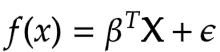
We can also generalize the above equation for multiple variables using a matrix of feature vectors. In this way, we will be finding the best fitting multidimensional hyperplane instead of a single line as is the case with most real-world data.
The entire goal of Least Square Regression is to find out the optimal value of the coefficients i.e. beta that minimises measurement of error. And makes reasonably good predictions on unseen data. And we can achieve this by minimising the residual sum of squares. It is the sum of the squares of the difference between the output and linear regression estimates. Given by
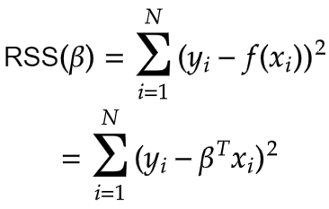
This is our cost function. The Maximum Likelihood Estimates for the beta that minimises the residual sum of squares (RSS) is given by
The focal point of everything till now is that in frequentist linear regression beta^ is a point estimate as opposed to the Bayesian approach where the outcomes are distributions.
Bayesian Framework
Before getting to the Bayesian Regression part let’s get familiar with the Bayes principle and know-how it does what it does? I suppose we are all a little familiar with the Bayes theorem. Let’s have a look at it.
The equation is given as
posterior = likelihood * prior / evidence
Prior probability, in Bayesian statistical inference, is the probability of an event occurring before new data is collected. In other words, it represents the best rational assessment of the probability of a particular outcome based on current knowledge before an experiment is performed.
The posterior probability is the revised probability of an event occurring after taking into consideration the new information. The posterior probability is calculated by updating the prior probability using Bayes’ theorem. In statistical terms, the posterior probability is the probability of event A occurring given that event B has occurred.
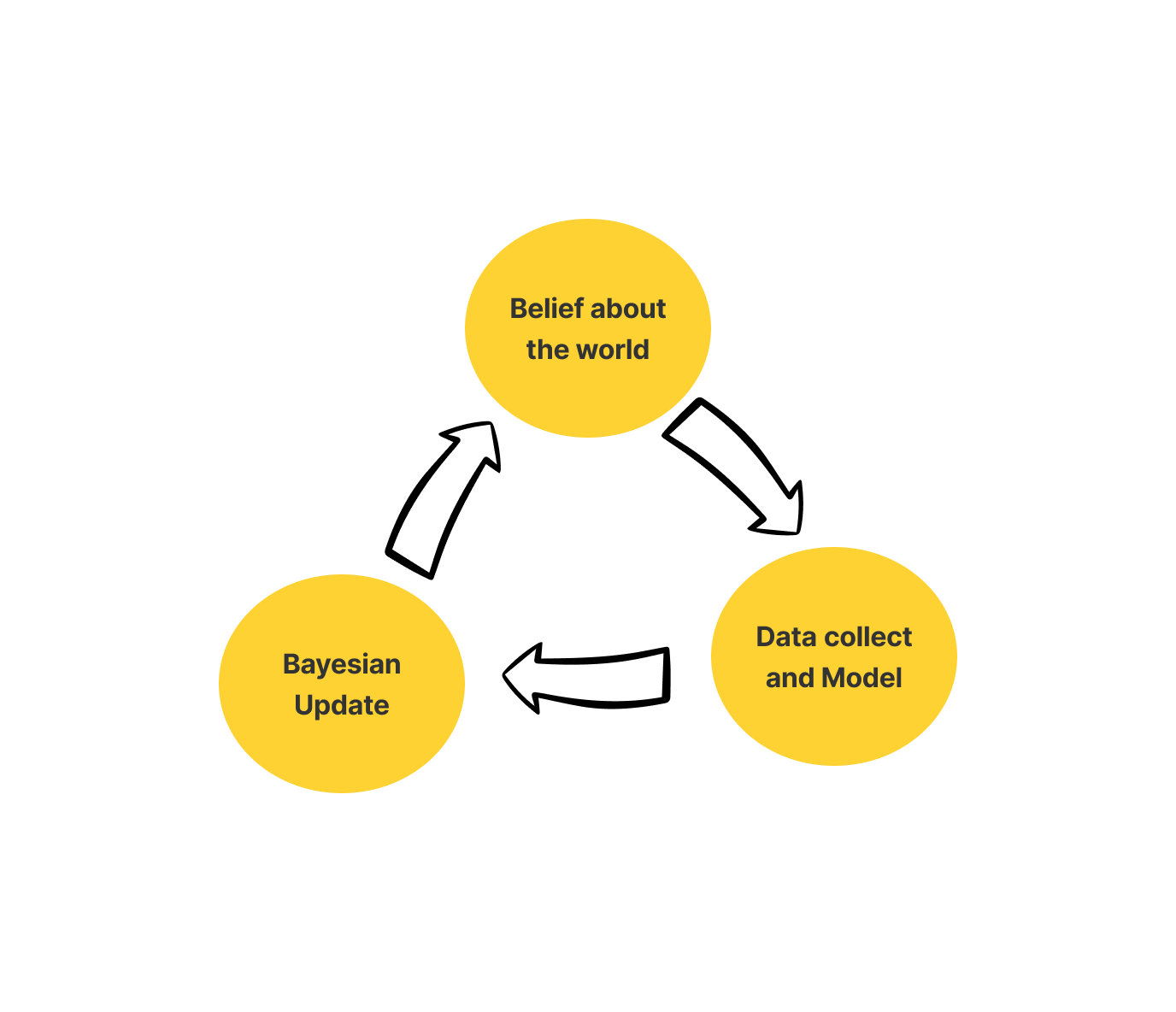
To sum it up the Bayesian framework has three basic tenets. These basic tenets outline the entire structure of Bayesian Frameworks.
- Belief: Belief about the world includes Prior and Likelihood
- Model: Collect data and use probability to update the model.
- Update: Update your belief as per your model
Let’s try to understand this through a simple example.
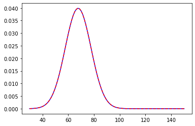
We are in a college and we want to measure the average height of male students. Now to make the Bayesian work we need a prior assumption regarding the process at hand. This is probably one of the best things in Bayesian Frameworks that it leaves enough room for one’s own belief, making it more intuitive in general. So to find the prior we must have some knowledge regarding the experiment. In our example, we will use let’s say the average height of males in that country. Let it be 67.73 inches with a standard deviation of 7. The distribution will look something like this
We centred the distribution at 67.73 with a standard deviation of 7. Now, we asked around and some good guys volunteered us and gave us their input. The first guy’s height was 76.11 inches. Now that we have new data we will update the posterior distribution.
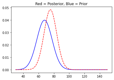
You can see the plot has shifted to the right as was obvious. We will now move on and collect some more data and update our posterior distribution accordingly.
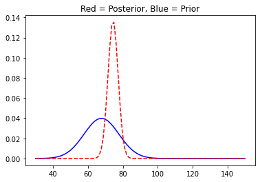
With more data, the posterior distribution starts to shrink in size as the variance of the distributions reduces. And it is quite similar to the way we experience things with more information at our disposal regarding a particular event we tend to make fewer mistakes or the likelihood of getting it right improves. Our brain works just as Bayesian Updating.
In a frequentist setting, the same problem could have been approached differently or we can say rather straightforward as we will only need to calculate the mean or median and desired confidence interval of our estimate. So, the question is why would someone go the extra mile to calculate these prior, posterior distributions and not just calculate the direct estimates? The sole reason for this is the increased interpretability of the model we now have a whole distribution of the quantity of interest rather than an estimate. So, now we can directly say about the probability of our estimates. But in a frequentist approach, the best we could do is to find a confidence interval of our estimates and these two terms, however similar they sound, are fundamentally different from each other.
A Confidence Interval is a measure of uncertainty around the true estimate. It is the combination of values above and below the true parameter which suggests that for a 95% confidence interval if we draw n samples from the population then 95% of the time the true (unknown) parameter will be captured by the said interval. But we cannot say that there is a 95% probability that the true parameter lies in that particular interval.
But with a Bayesian posterior distribution, we can very well predict the probability of true parameter within an interval and this is called Credible Interval. And it can do that because the parameters are considered random in the Bayesian framework. And this thing is very powerful for any kind of research analysis.
Bayesian Linear Regression
We just learned how the entire thought process that goes behind the Bayesian approach is fundamentally different from that of the Frequentist approach. As we saw in the previous section OLS estimates a single value for a parameter that minimises the cost function, but in a Bayesian world instead of single values, we will estimate entire distributions for each parameter individually. That means every parameter is a random value sampled from a distribution with a mean and variance. The standard syntax for Bayesian Linear Regression is given by
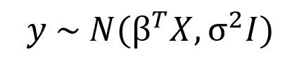
Here, as you can see the response variable is not anymore a point estimate but a normal distribution with a mean 𝛽TX and variance sigma2I, where 𝛽TX is the general linear equation in X and I is the identity matrix to account for the multivariate nature of the distribution.
Bayesian calculations more often than not are tough, and cumbersome. It takes far more resources to do a Bayesian regression than a Linear one. Thankfully we have libraries that take care of this complexity. For this article, we will be using the PyMC3 library for calculation and Arviz for visualizations. So, let’s get started.
Bayesian Analysis with PyMC3 and Arviz
So, far we learned the workings of Bayesian updating. Now. in this section we are going to work out a simple Bayesian analysis of a dataset. For this article, to keep things straight forward we are going to use the height-weight dataset. This is a fairly simple dataset and here we will be using weight as the response variable and height as a predictor variable.
So, before going full throttle at it let’s get familiar with the PyMC3 library. This powerful Probabilistic Programming Framework was designed to incorporate Bayesian techniques in data analysis processes. PyMC3 provides Generalized Linear Modules(GLM) to extend the functionalities of OLS to other regression techniques such as Logistic Regression, Poisson Regression etc. The response or outcome variable is related to predictor variables via a link function. And its usability is not limited to normal distribution but can be extended to any distribution from the ”exponential family“.
Now we are all set for the real deal.
Importing Libraries and Data
For dealing with data we will be using Pandas and Numpy, Bayesian modelling will be aided by PyMC3 and for visualizations, we will be using seaborn, matplotlib and arviz. Arviz is a dedicated library for Bayesian Exploratory Data Analysis. Which has a lot of tools for many statistical visualizations.
import pandas as pd
import numpy as np
import matplotlib.pyplot as plt
import seaborn as sns
import pymc3 as pm
import arviz as az
As I said earlier we will be using a simple Height-Weight dataset.
df = pd.read_csv('/content/weight-height.csv')
df.head()
Scaling Data
Scaling data is always deemed a good practice. We do not want our data to wander, scaling data will help contain data within a small boundary while not losing its original properties. More often than not variation in the outcome and predictors are quite high and samplers used in the GLM module might not perform as intended so it’s good practice to scale the data and it does no harm anyway.
from sklearn.preprocessing import StandardScaler
scale = StandardScaler()
dt = df.loc[:1000]
dt = pd.DataFrame(scale.fit_transform(dt.drop('Gender', axis=1)), columns=['x','y'])
Frequentist Linear Regression
from sklearn.linear_model import LinearRegression
lr = LinearRegression()
lr.fit(np.array(dt.Height).reshape(-1,1), dt.Weight)
print(lr.coef_,lr.intercept_)
output: [0.84468401] -1.8287518566290025e-15
We will use these estimates later on.
Modeling Data
PyMC3 uses GLM (Generalized Linear Models) to operate on data. It is required to specify a model with a “with” context manager. We will use MAP (Maximum A Posteriori) as a starting point for MCMC and finally will use the No-U-Turn sampler to calculate the trace. The idea behind MCMC is that Bayesian Models become intractable in high dimensional space an efficient search method is necessary to carry out sampling that is how we got MCMC. It has a collection of algorithms that are used for sampling variables.
my_model = pm.Model()
with my_model:
    pm.glm.GLM(x=dt.x,y=dt.y, family = pm.glm.families.Normal())
    #using MAP(MAximum A Posteriori as initial value for MCMC sampler)
    start = pm.find_MAP()
    trace = pm.sample(1000,chains=2, return_inferencedata=False)
.png)
This will return a trace object. A tracing object is nothing but a collection of dictionaries consisting of posterior predicted values. The values that are used to construct the ultimate posterior distributions.
print(list(trace))
.png)
The start gives the starting point for MCMC sampling. The MAP estimates the most common value as the point estimate which is also the mean for a normal distribution. The interesting part is the value is the same as the Maximum Likelihood Estimate.
print(start)
{'Intercept': array(-1.84954468e-15),
 'sd': array(0.53526373),
 'sd_log__': array(-0.6249957),
 'x': array(0.84468401)}
Posterior Predictive
Next up we calculate the posterior predictive estimates. And this is not the same as the posterior we saw earlier. The posterior distribution “is the distribution of an unknown quantity, treated as a random variable, conditional on the evidence obtained” (Wikipedia). It’s the distribution that explains your unknown, random, parameter. While the posterior predictive distribution is the distribution of possible unobserved values conditional on the observed values (Wikipedia).
with my_model:
    ppc = pm.sample_posterior_predictive(
        trace, random_seed=42, progressbar=True
    )
Converting Trace Objects to Inference Object
A lot of arviz methods work fine with trace objects while a number of them do not. In future releases PyMC3 most likely will return inference objects. We will also include our posterior predictive estimates in our final inference object.
with my_model:
    trace_updated = az.from_pymc3(trace, posterior_predictive=ppc)
Trace Plots
az.style.use("arviz-darkgrid")
with my_model:
  az.plot_trace(trace_updated, figsize=(17,10), legend=True)
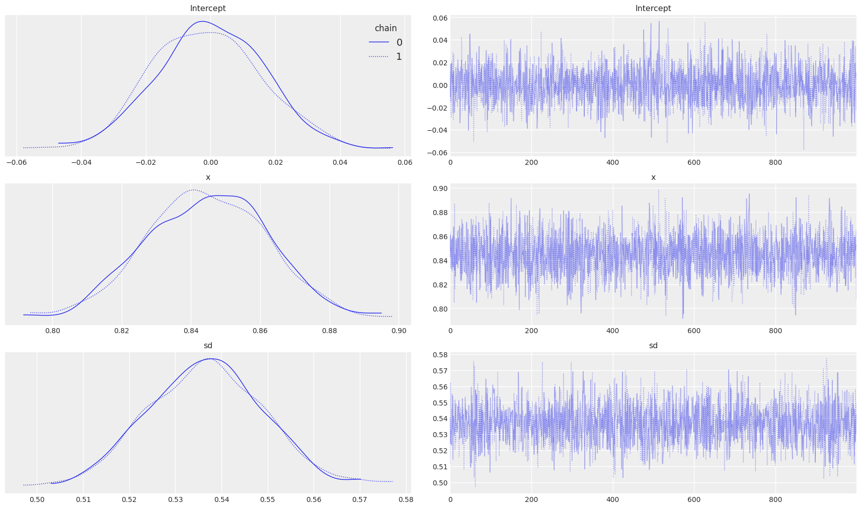
On the left side of the plot, we can observe the posterior plots of our parameters and distribution for standard deviation. Interestingly the mean of the parameters is almost the same as that of the Linear Regression we saw earlier.
Posterior Plots
az.style.use("arviz-darkgrid")
with my_model:
  az.plot_posterior(trace_updated,textsize=16)
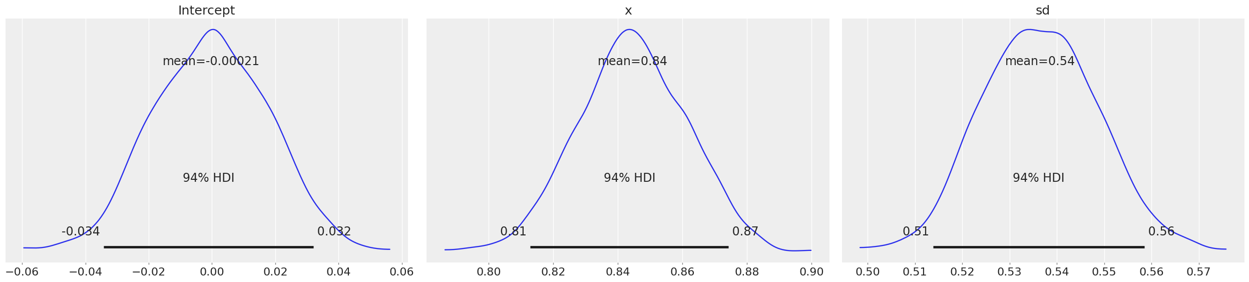
Now if you observe the means of intercept and variable x are almost the same as what we estimated from frequentist Linear Regression. Here, HDI stands for Highest Probability Density, which means any point within that boundary will have more probability than points outside.
Posterior Predictive Check
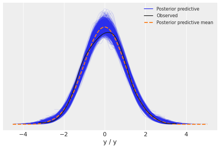
Posterior predictive plots help us visualize if the model can reproduce the patterns observed in the real data.
az.style.use("arviz-darkgrid")
with my_model:
  az.plot_ppc(trace_updated)
We will now visualize all the linear plots for the posterior parameter and frequentist linear regression line. And if you were wondering why we renamed our variables to x and y is because of this plot as post_predictive_glm() has it hardcoded that any variable named other than x when passed will throw a keyword error. So, this was a workaround.
with my_model:
  sns.lmplot(x="x", y="y", data=dt, size=10, fit_reg=True)
  plt.xlim(0, 1)
  plt.ylim(-0.2, 1)
  beta_0, beta_1 = lr.intercept_, lr.coef_ #estimates of OLS
  pm.plot_posterior_predictive_glm(trace_updated, samples=200)
  y = beta_0 + beta_1*dt.x
  plt.plot(dt.x, y, label="True Regression Line", lw=2, c="red")
  plt.legend(loc=0)
  plt.show()
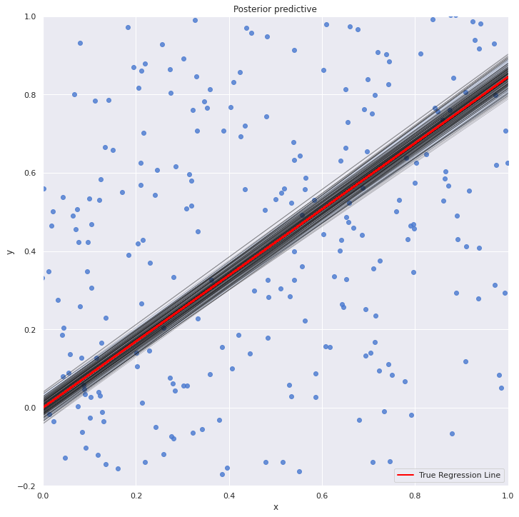
The OLS line is pretty much at the middle of all the line plots from the posterior distribution.
Where Do We Use It?
So, far so good. We learnt the basics of Bayesian Linear Regression. But where in the real world this can be implemented? Well, there could be numerous such instances where we can use Bayesian Linear Regression. In any such situation where we have limited historical data regarding some events, we can incorporate the prior data into the model to get better results.
For example, a supermarket wishes to launch a new product line this holiday season and the management intends to know the overall sales forecast of the particular product line. In a situation like this where we do not have enough historical data to efficiently forecast sales, we can always incorporate the average effect of a similar product line as the prior for the new products’ holiday season effects. And the prior will get updated upon seeing new data. So, we will get a reasonable Holiday sale forecast for the new product line.
In hierarchical modelling Bayesian regression is used where we need to account for the individual as well as group effect of the variables. For example, modelling the SAT scores of students from different schools. Here, the outcomes depend both on individual variables (students) as well as the school level variables(environment, socio-economics etc). In cases like this, we can use the concept of hierarchical priors to account for both individual and group effects. More reading on this can be found here.
And one of the added advantages of Bayesian is that it does not require regularization. The prior itself work as a regularizer. When we take a prior with a tight distribution or a small standard deviation it signals we have a strong belief in the prior. And it takes a lot of data to shift the distribution away from prior parameters. It does the work of a regularizer in the frequentists approach though they are implemented differently (one through optimisation and the other through sampling). This reduces the hassle of using extra regularization parameters for over parameterized models.
Pros and Cons
Before winding up we must discuss the pros and cons of the Bayesian Approach and when should we use it and when should not.
Pros
- Increased interpretability
- Being able to incorporate prior beliefs
- Being able to say the percentage probability of any point in the posterior distribution
- Can be used for Hierarchical or multilevel models
Cons
- Slower compared to frequentist. where performance and speed are essential Bayesian does a pretty not good job.
- May not perform as desired in high dimensional space
- A bad prior belief may distract the model
Conclusion
Throughout the article, we explored the Bayesian approach to regression analysis. The key thing to notice here is that in OLS we will only be able to find the point estimate, a single value for each coefficient while the only term random is the residual term. While in Bayesian Approach we are getting individual distributions for each predictor variable. Which subsequently enables us to make better judgements. We can predict the percentage probability of an estimate which is very powerful and not there in the frequentist statistics.
The media shown in this article is not owned by Analytics Vidhya and is used at the Author’s discretion.
Meet your author Sunil kumar Dash, a developer and a writer. Has diverse interests in tech, pop culture, wellness, philosophy and Anime. Exploring underrated music is his hobby. And loves to doom scroll Twitter when bored.


