This article was published as a part of the Data Science Blogathon.
Introduction to Linear Regression
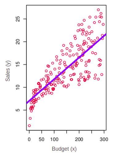
Linear regression is a statistical method that presumes a linear relationship between the input and the output variables. In the given example above we can see that budget is the input variable “x” and sales is the output variable “y”. In this example, the linear regression produces a linear model (blue) which presumes that there is a linear relationship between the input variable “budget” and the output variable “sales”.
Moving Beyond Linear Regression
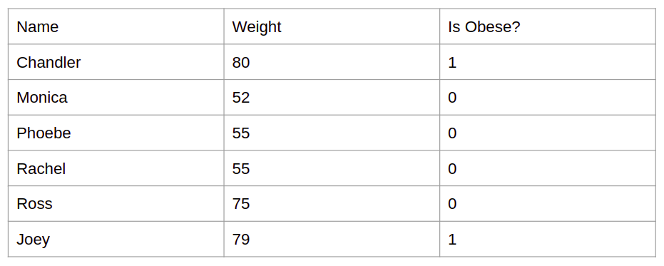
Now, take a look at this example instead. What we are seeing here is that we have a bunch of people and their corresponding weights. And they are not just a bunch of ordinary people but our “friends”. You can see that we have listed the approximate weights of all the friends’ characters. Monica, Phoebe, and Rachel seem to have the weights on the lower side. Similarly, Chandler, Joey, and Ross have higher weights. Notice that there is a third column called “obese” which has two options 0 or 1. Here, 0 indicates that the corresponding person is not obese (overweight). On the other hand, 1 represents he or she is obese. So, of all the friends, Chandler and Joey seem to be slightly overweight. If we plot this information over a graph we will see a figure that looks like this.
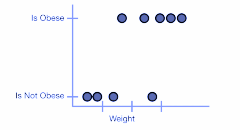
Because of two classes (obese and non-obese), the graph has data points that only have values of 0 and 1. Is it possible to apply linear regression in this dataset like in the earlier example of linear regression? Well, maybe. We can make an assumption that there could be a linear relationship between the x and y-axis. However, when we try to create a linear model we can quickly find that the model could not be an accurate representation of that dataset.
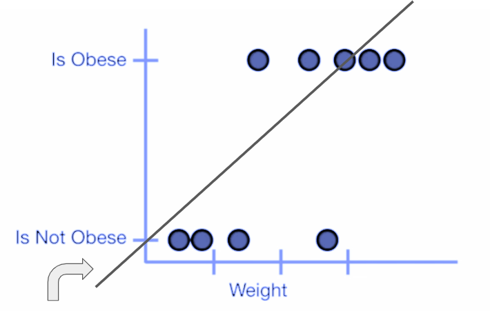
First of all the linear model is responsible for creating too much residue/error because the distance between the predicted line and individual data points in this data set is too high. And secondly, we can also analyze that this linear equation is predicting the negative axis which doesn’t make any sense. The weight having a negative value has no meaning. Similarly, the y-axis contains only 2 classes in the form of obese and non-obese. Therefore the negative axis of “y” also holds no meaning. So it’s safe to make an assumption that linear models cannot accurately model such datasets.
The Logistic Model
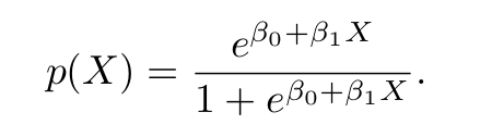
Now that we are certain that we need a better option than a linear model, we introduce the concept of the logistic model. Rather than modelling y or the response directly, the logistic regression model predicts the probability that y belongs to a particular category. Therefore in our obesity example, one might predict that obesity is “yes” for any individual whose probability of weight is greater than 0.5. If we go for a more conservative approach we can also lower the threshold such that the probability of weight greater than 0.1 would be termed as obese.
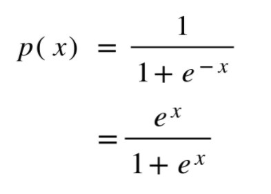
In the linear model, we considered using a linear regression line to represent these probabilities in the form of the equation y = mx + b. However, in the logistic model, we use a logistic function or a sigmoid function to model our data. Mathematically the logistic model can be represented by the following equation.
<img width=”268px;” height=”81px;” src=”https://lh6.googleusercontent.com/CFfXCl_jsVE59iTQZeKU5mSfwG3qlPSXa9AW7WZoGn0G0ezmXX0q2V6PF1icxqqsLbCJ71REzS1HLaMDyczW_CMIkkxHgw0eVyBEr9CNYVw_QKHOnBdCI9F21ee29TYB3L4PRjXaYSKZ” title=”p open parentheses x close parentheses space equals space fraction numerator 1 over denominator 1 plus e to the power of negative x end exponent end fraction” alt=”px = 11+e-x”>
After a little bit of tweaking, we get this equation.
When we plot out the corresponding sigmoid graph we get something like this.
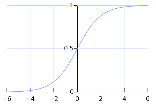
Notice that the x-axis is spread from minus infinity to plus infinity and the y axis only contains 0 and 1. It means that the sigmoid function takes the value of the x-axis and squeezes it between 0 and 1 (doesn’t matter how large the x-axis number is). This is because the sigmoid graph creates an asymptote on the y = 1 line as the value approaches the positive infinity. Likewise, the graph also makes asymptotes on the y = 0 line. It means that the corresponding value of the function will tend to reach zero when the x-axis value tends to be minus infinity. So now as we look back on our obesity data we can intuitively say that this data would need a sigmoid function in order to represent these data points correctly. But how do we achieve this? It’s not that we are going to draw an arbitrary curve and make an assumption that it is the best fit. We didn’t follow this approach in the linear model. Remember that in the linear model we tend to find the line which has the minimum amount of error/residue. Therefore in the logistic regression as well we need to figure out a way that would minimize our error so that the data points are represented correctly by our sigmoid function. So what do you think we need to do to achieve this?
We will use the concept of maximum likelihood. But before we are jumping into the concept of likelihood I would like to introduce another concept called the “odds”. Mathematically speaking odds can be described as the ratio of the probability of an event’s occurrence over the probability of the event’s non-occurrence. Let’s say we have the sigmoid function equation like this.
After a bit of tweaking, we can get an equation that looks like this.
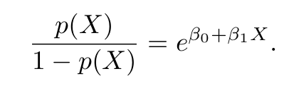
Notice that on the left-hand side of the equation we are getting the ratio of the probability of occurrence of something over the probability of non-occurrence which is also known as the odds. Suppose I tell you that the odds of Arsenal football club qualifying for the Champions League next season is 5 is to 3. It means that on 5 chances, the team would qualify whereas on three chances they would not qualify. It means that the odds are in their favour and not against them.
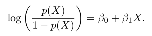
But let’s back off for a moment and rethink why we are calculating the odds while looking into the logistic regression. It turns out that we are deriving odds in order to derive something called log-odds or logit. Logit is nothing but the natural log of odds and it can be achieved by taking logs on both sides of the previous equation.
Now that we have figured out a way to find the log odds we can finally dive into the concept of maximum likelihood.
We will continue digging into the concepts of Maximum Likelihood in detail in the upcoming article Logistic Regression and Maximum Likelihood: Explained Simply (Part II)
End Notes
- The linear regression cannot accurately model the classification data.
- The idea of logistic regression is to be applied when it comes to classification data.
- Logistic regression is used for classification problems.
- It fits the squiggle by something called “maximum likelihood”.
Hope you liked my article on Linear Regression. Read more articles on the blog.
About The Author
Hi there! My name is Akash and I’ve been working as a Python developer for over 4 years now. In the course of my career, I began as a Junior Python Developer at Nepal’s biggest Job portal site. Later, I was involved in Data Science and research at Nepal’s first ride-sharing company, Tootle. Currently, I’ve been actively involved in Data Science as well as Web Development with Django.
You can find my other projects on:
https://github.com/akashadhikari
Connect me on LinkedIn
https://www.linkedin.com/in/akashadh/
Email: [email protected] | [email protected]
Image sources:
Image 1: https://www.statlearning.com/
Image 4: https://en.wikipedia.org/wiki/Logistic_function
The media shown in this article is not owned by Analytics Vidhya and are used at the Author’s discretion.


