Autoregressive models are one of the most important ideas in time series forecasting and sequence modeling. The name may sound technical at first, but the concept is surprisingly intuitive.
An autoregressive model predicts the next value by looking at previous values.
That is the core idea.
For example, tomorrow’s temperature may depend on the temperatures from the last few days. Next month’s sales may depend on sales from previous months. The next word in a sentence may depend on the words that came before it — the main idea powering LLMs.
In all these cases, the model is using the past to predict what comes next.
Table of contents
What Does Autoregressive Mean?
The word autoregressive has two parts.
Auto means self.
Regressive means predicting a variable using other variables.
So, autoregressive means predicting a variable using its own previous values.
In simple terms:
An autoregressive model predicts the current or next value based on past values of the same variable.
Suppose we are forecasting daily website traffic. If traffic has been increasing steadily over the past few days, an autoregressive model can use that pattern to estimate tomorrow’s traffic.
For example:
Monday: 1000 visits
Tuesday: 1100 visits
Wednesday: 1200 visits
Thursday: ?
The model may predict around 1300 visits for Thursday because the recent pattern suggests an increase of about 100 visits per day.
Of course, real-world data is rarely this clean. There may be weekends, campaigns, holidays, outages, or random noise. But the basic idea remains the same: the past contains useful information about the future.
The Basic Autoregressive Model
A simple autoregressive model can be written as:
xₜ = c + φ₁xₜ₋₁ + εₜ
This is called an AR(1) model.
Click here to see the breakdown of the formula
- xₜ is the value we want to predict at time t.
- xₜ₋₁ is the previous value.
- c is a constant.
- φ₁ is a coefficient that tells us how strongly the previous value affects the current value.
- εₜ is the error term, or random noise.
The model says that the current value is a combination of:
- a constant,
- the previous value,
- and some random error.
So, an AR(1) model predicts the current value using only one past observation.
The General Autoregressive Model
If we use more than one previous value, we get a more general model:
xₜ = c + φ₁xₜ₋₁ + φ₂xₜ₋₂ + … + φₚxₜ₋ₚ + εₜ
This is called an AR(p) model.
Here, p tells us how many past values the model uses.
Examples:
- AR(1) uses one previous value.
- AR(2) uses two previous values.
- AR(5) uses five previous values.
So, if we say a model is AR(3), it means the model predicts the current value using the last three observations.
A Simple Example
Imagine you are trying to predict the demand for a product.
The sales for the past five days were:
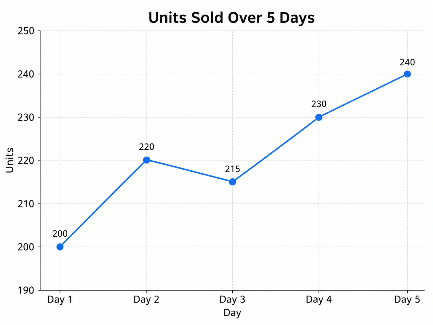
An autoregressive model looks at these past sales values and tries to learn the relationship between them.
It may learn that sales today are strongly related to sales yesterday. It may also find that sales from two or three days ago still carry some useful signal.
Once the model learns this relationship, it can forecast Day 6.
This is useful because many real-world patterns have memory. Sales, stock prices, temperature, electricity usage, website traffic, and customer demand often depend on what happened recently.
Why Are Autoregressive Models Useful?
Autoregressive models are useful because they are simple, interpretable, and powerful for many forecasting problems.
They work especially well when recent history is a good predictor of the near future.
For example, if electricity consumption has been high for the past few hours, it may remain high in the next hour. If a stock has shown a certain pattern recently, traders may try to use that information for short-term forecasting. If a website has high traffic today, it may continue to have high traffic tomorrow.
Another advantage is explicability.
In many machine learning models, it can be hard to understand exactly why the model made a prediction. But autoregressive models are easier to explain because the prediction is directly tied to previous values.
We can look at the coefficients and understand how much each past value contributes to the prediction.
Where Are Autoregressive Models Used?
Autoregressive models are widely used in time series analysis.
Some common applications include:
- Sales forecasting
- Demand prediction
- Stock price analysis
- Weather forecasting
- Economic forecasting
But autoregressive modeling is not limited to traditional time series.
It is also a key idea behind language models.
Autoregressive Models in Language Modeling
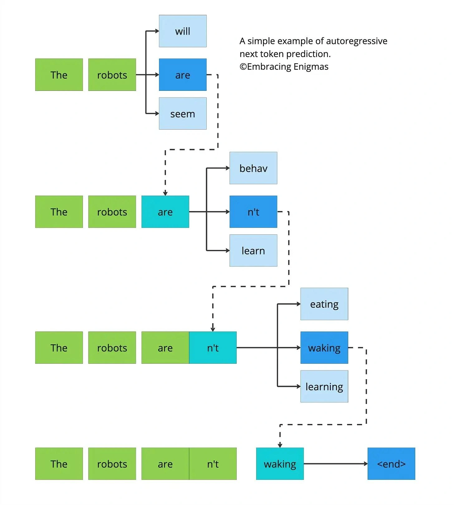
In natural language processing, autoregressive models generate text one token at a time.
A token can be a word, part of a word, or even a character, depending on the model. This is the central concept powering Large Language Models.
For example, consider this sentence:
The cat sat on the
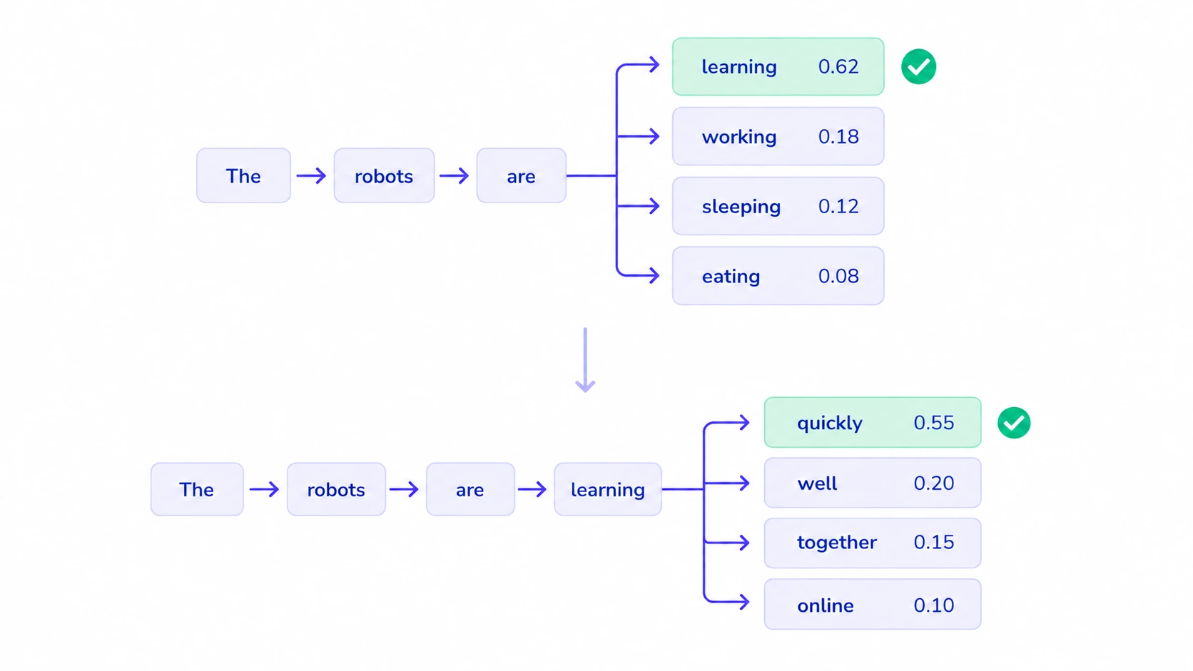
An autoregressive language model predicts the next token based on the previous tokens.
It may predict:
mat
Then the sentence becomes:
The cat sat on the mat
Now the model uses the updated sentence to predict the next token. This continues one step at a time.
The probability of a sentence can be written as:
P(w₁, w₂, w₃, …, wₙ) = P(w₁) × P(w₂ | w₁) × P(w₃ | w₁, w₂) × … × P(wₙ | w₁, …, wₙ₋₁)
This means each word is predicted based on the words before it.
The model does not generate the whole sentence at once. It builds the sentence step by step (sequentially), using previous tokens as context.
Autoregressive vs Non-Autoregressive Models
The difference between Autoregressive and Non-Autoregressive models are:
| Point | Autoregressive Models | Non-Autoregressive Models |
| Generation | One output at a time | Multiple outputs at once |
| Dependency | Depends on previous outputs | Less dependent on previous outputs |
| Speed | Slower | Faster |
| Strength | Captures sequence well | Better for parallel generation |
| Example | Predicts words token by token | Generates several tokens together |
Limitations of Autoregressive Models
Here are the limitations of Autoregressive Models:
- Autoregressive models rely heavily on past values, so they may struggle when unexpected events occur.
- A sudden sales jump due to a viral campaign may not be captured unless external variables are included.
- A drop in demand caused by supply issues may not be understood from past demand values alone.
- Traditional autoregressive models are mostly linear and assume the current value is a linear combination of past values.
- Many real-world patterns are more complex, so advanced models like VAR, LSTMs, Transformers, and other deep learning models can be useful.
Conclusion
Autoregressive models remain one of the clearest ways to understand forecasting and sequence modeling. By learning from past values, they offer a simple yet powerful framework for predicting what comes next, whether in sales, sensor data, or language.
While they may miss sudden shocks, nonlinear behavior, or outside influences, their value as a starting point is undeniable. For anyone exploring time series or generative AI, they provide a strong foundation to build on.
TLDR: Autoregressive models use the past to predict the future.
I specialize in reviewing and refining AI-driven research, technical documentation, and content related to emerging AI technologies. My experience spans AI model training, data analysis, and information retrieval, allowing me to craft content that is both technically accurate and accessible.


