The success of machine learning pipelines depends on feature engineering as their essential foundation. The two strongest methods for handling time series data are lag features and rolling features, according to your advanced techniques. The ability to use these techniques will enhance your model performance for sales forecasting, stock price prediction, and demand planning tasks.
This guide explains lag and rolling features by showing their importance and providing Python implementation methods and potential implementation challenges through working code examples.
Table of contents
What is Feature Engineering in Time Series?
Time series feature engineering creates new input variables through the process of transforming raw temporal data into features that enable machine learning models to detect temporal patterns more effectively. Time series data differs from static datasets because it maintains a sequential structure, which requires observers to understand that past observations impact what will come next.
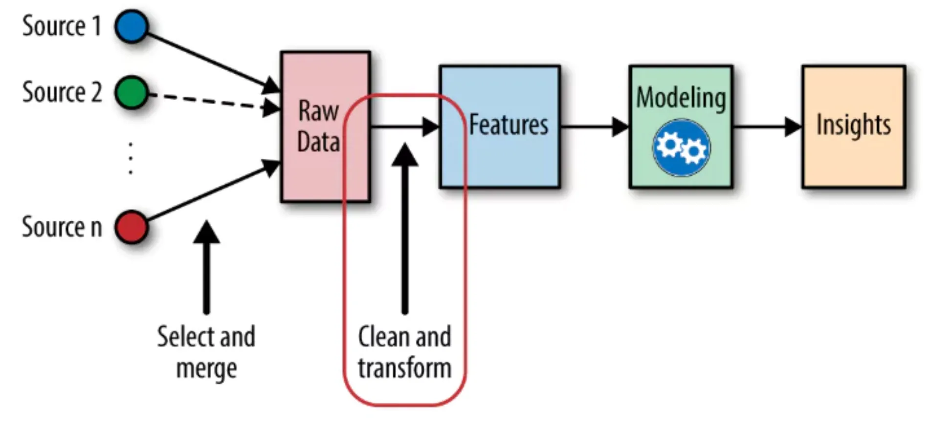
The conventional machine learning models XGBoost, LightGBM, and Random Forests lack built-in capabilities to process time. The system requires specific indicators that need to show past events that occurred before. The implementation of lag features together with rolling features serves this purpose.
What Are Lag Features?
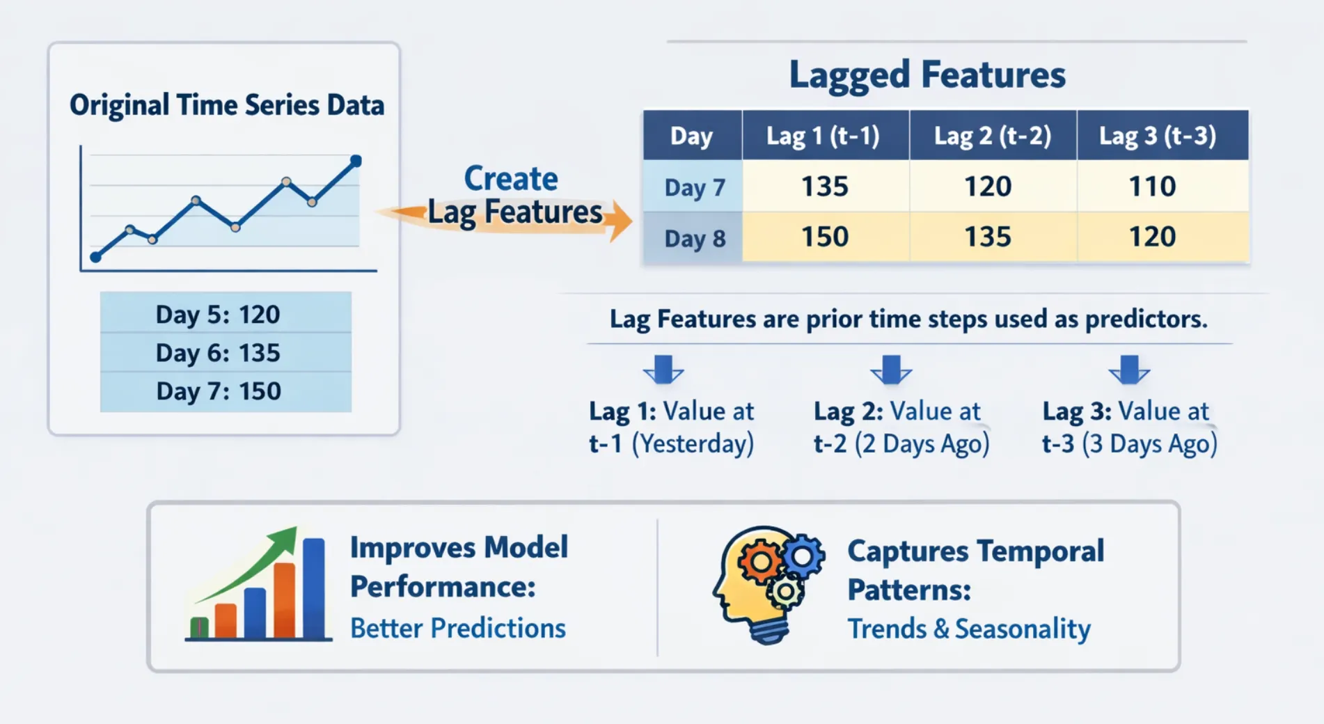
A lag feature is simply a past value of a variable that has been shifted forward in time until it matches the current data point. The sales prediction for today depends on three different sales information sources, which include yesterday’s sales data and both seven-day and thirty-day sales data.
Why Lag Features Matter
- They represent the connection between different time periods when a variable shows its past values.
- The method allows seasonal and cyclical patterns to be encoded without needing complicated transformations.
- The method provides simple computation together with clear results.
- The system works with all machine learning models that use tree structures and linear methods.
Implementing LAG Features in Python
import pandas as pd
import numpy as np
# Create a sample time series dataset
np.random.seed(42)
dates = pd.date_range(start='2024-01-01', periods=15, freq='D')
sales = [200, 215, 198, 230, 245, 210, 225, 260, 275, 240, 255, 290, 305, 270, 285]
df = pd.DataFrame({'date': dates, 'sales': sales})
df.set_index('date', inplace=True)
# Create lag features
df['lag_1'] = df['sales'].shift(1)
df['lag_3'] = df['sales'].shift(3)
df['lag_7'] = df['sales'].shift(7)
print(df.head(12))
Output:
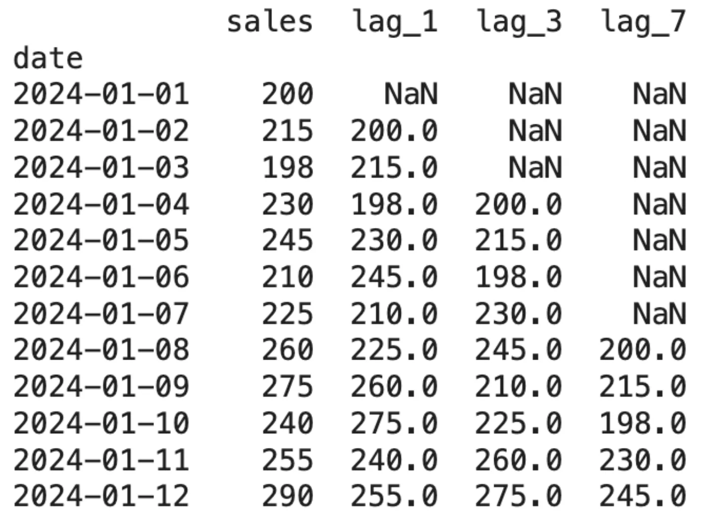
The initial appearance of NaN values demonstrates a form of data loss that occurs because of lagging. This factor becomes crucial for determining the number of lags to be created.
Choosing the Right Lag Values
The selection process for optimal lags demands scientific methods that eliminate random selection as an option. The following methods have shown successful results in practice:
- The knowledge of the domain helps a lot, like Weekly sales data? Add lags at 7, 14, 28 days. Hourly energy data? Try 24 to 48 hours.
- Autocorrelation Function ACF enables users to determine which lags show significant links to their target variable through its statistical detection method.
- The model will identify which lags hold the highest significance after you complete the training procedure.
What Are Rolling (Window) Features?
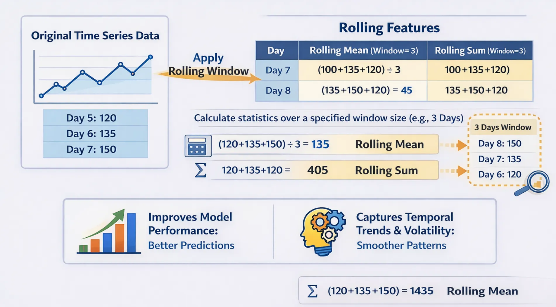
The rolling features function as window features that operate by moving through time to calculate variable quantities. The system provides you with aggregated statistics, which include mean, median, standard deviation, minimum, and maximum values for the last N periods instead of showing you a single past value.
Why Rolling Features Matter?
The following features provide excellent capabilities to perform their designated tasks:
- The process eliminates noise elements while it reveals the fundamental growth patterns.
- The system enables users to observe short-term price fluctuations that occur within specific time periods.
- The system enables users to observe short-term price fluctuations that occur within specific time periods.
- The system identifies unusual behaviour when present values move away from the established rolling average.
The following aggregations establish their presence as standard practice in rolling windows:
- The most common method of trend smoothing uses a rolling mean as its primary method.
- The rolling standard deviation function calculates the degree of variability that exists within a specified time window.
- The rolling minimum and maximum functions identify the highest and lowest values that occur during a defined time interval/period.
- The rolling median function provides accurate results for data that includes outliers and exhibits high levels of noise.
- The rolling sum function helps track total volume or total count across time.
Implementing Rolling Features in Python
import pandas as pd
import numpy as np
np.random.seed(42)
dates = pd.date_range(start='2024-01-01', periods=15, freq='D')
sales = [200, 215, 198, 230, 245, 210, 225, 260, 275, 240, 255, 290, 305, 270, 285]
df = pd.DataFrame({'date': dates, 'sales': sales})
df.set_index('date', inplace=True)
# Rolling features with window size of 3 and 7
df['roll_mean_3'] = df['sales'].shift(1).rolling(window=3).mean()
df['roll_std_3'] = df['sales'].shift(1).rolling(window=3).std()
df['roll_max_3'] = df['sales'].shift(1).rolling(window=3).max()
df['roll_mean_7'] = df['sales'].shift(1).rolling(window=7).mean()
print(df.round(2))
Output:
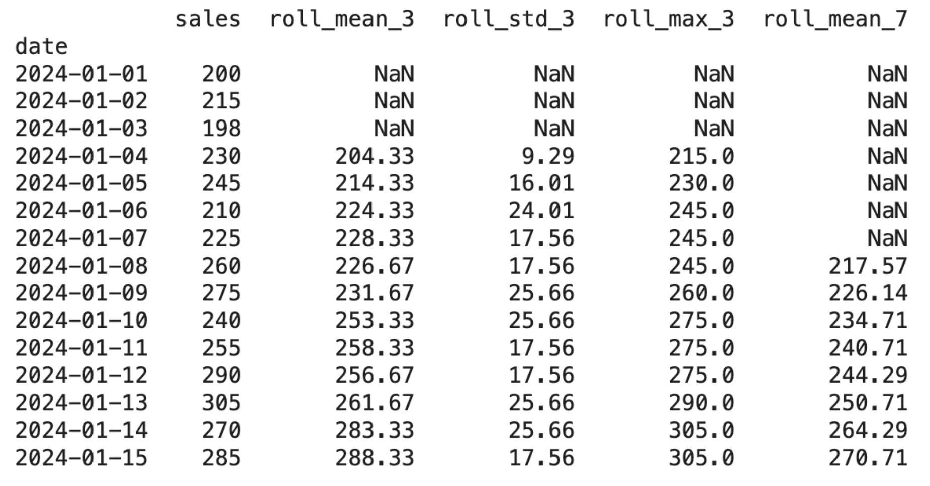
The .shift(1) function must be executed before the .rolling() function because it creates a vital connection between both functions. The system needs this mechanism because it will create rolling calculations that depend exclusively on historical data without using any current data.
Combining Lag and Rolling Features: A Production-Ready Example
In actual machine learning time series workflows, researchers create their own hybrid feature set, which includes both lag features and rolling features. We provide you with a complete feature engineering function, which you can use for any project.
import pandas as pd
import numpy as np
def create_time_features(df, target_col, lags=[1, 3, 7], windows=[3, 7]):
"""
Create lag and rolling features for time series ML.
Parameters:
df : DataFrame with datetime index
target_col : Name of the target column
lags : List of lag periods
windows : List of rolling window sizes
Returns:
DataFrame with new features
"""
df = df.copy()
# Lag features
for lag in lags:
df[f'lag_{lag}'] = df[target_col].shift(lag)
# Rolling features (shift by 1 to avoid leakage)
for window in windows:
shifted = df[target_col].shift(1)
df[f'roll_mean_{window}'] = shifted.rolling(window).mean()
df[f'roll_std_{window}'] = shifted.rolling(window).std()
df[f'roll_max_{window}'] = shifted.rolling(window).max()
df[f'roll_min_{window}'] = shifted.rolling(window).min()
return df.dropna() # Drop rows with NaN from lag/rolling
# Sample usage
np.random.seed(0)
dates = pd.date_range('2024-01-01', periods=60, freq='D')
sales = 200 + np.cumsum(np.random.randn(60) * 5)
df = pd.DataFrame({'sales': sales}, index=dates)
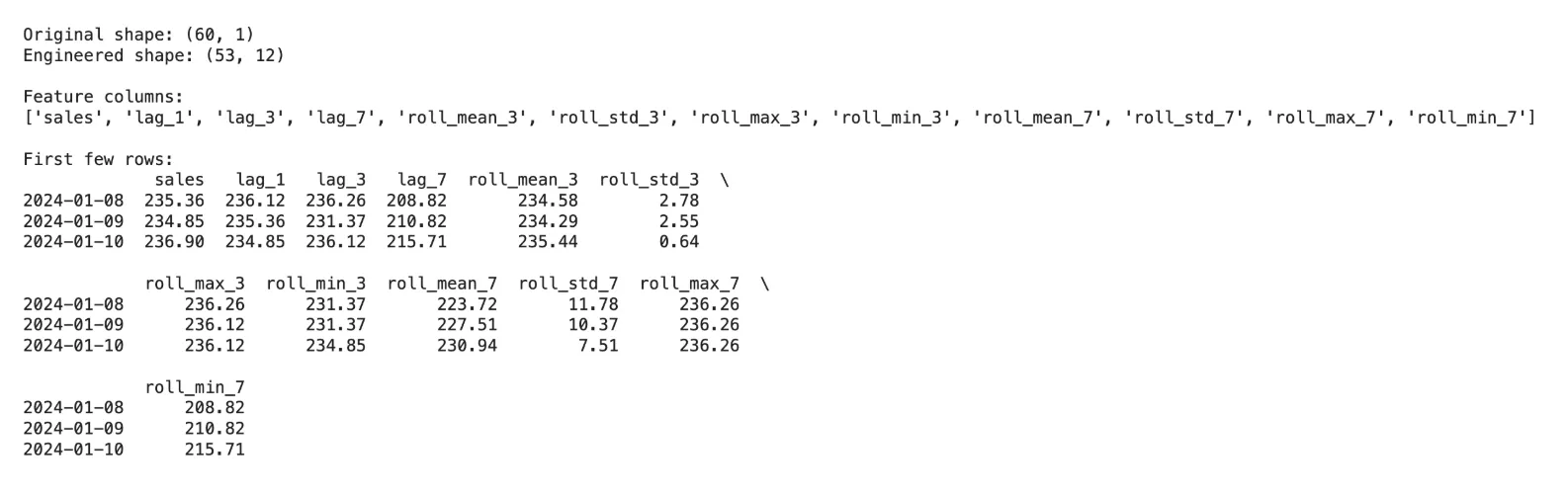
df_features = create_time_features(df, 'sales', lags=[1, 3, 7], windows=[3, 7])
print(f"Original shape: {df.shape}")
print(f"Engineered shape: {df_features.shape}")
print(f"\nFeature columns:\n{list(df_features.columns)}")
print(f"\nFirst few rows:\n{df_features.head(3).round(2)}")Output:
Common Mistakes and How to Avoid Them
The most severe error in time series feature engineering occurs when data leakage, which reveals upcoming data to testing features, leads to misleading model performance.
Key mistakes to watch out for:
- The process requires a .shift(1) command before starting the .rolling() function. The current observation will become part of the rolling window because rolling requires the first observation to be shifted.
- Data loss occurs through the addition of lags because each lag creates NaN rows. The 100-row dataset will lose 30% of its data because 30 lags require 30 NaN rows to be created.
- The process requires separate window size experiments because different characteristics need different window sizes. The process requires testing short windows, which range from 3 to 5, and long windows, which range from 14 to 30.
- The production environment requires you to compute rolling and lag features from actual historical data, which you will use during inference time instead of using your training data.
When to Use Lag vs. Rolling Features
| Use Case | Recommended Features |
|---|---|
| Strong autocorrelation in data | Lag features (lag-1, lag-7) |
| Noisy signal, need smoothing | Rolling mean |
| Seasonal patterns (weekly) | Lag-7, lag-14, lag-28 |
| Trend detection | Rolling mean over long windows |
| Anomaly detection | Deviation from rolling mean |
| Capturing variability / risk | Rolling standard deviation, rolling range |
Conclusion
The time series machine learning infrastructure uses lag features and rolling features as its essential components. The two methods establish a pathway from unprocessed sequential data to the organized data format that machine learning models require for their training process. The methods become the highest impact factor for forecasting accuracy when users execute them with precise data handling and window selection methods, and their contextual understanding of the specific field.
The best part? They provide clear explanations that require minimal computing resources and function with any machine learning model. These features will benefit you regardless of whether you use XGBoost for demand forecasting, LSTM for anomaly detection, or linear regression for baseline models.
Gen AI Intern at Analytics Vidhya
Department of Computer Science, Vellore Institute of Technology, Vellore, India
I am currently working as a Gen AI Intern at Analytics Vidhya, where I contribute to innovative AI-driven solutions that empower businesses to leverage data effectively. As a final-year Computer Science student at Vellore Institute of Technology, I bring a solid foundation in software development, data analytics, and machine learning to my role.
Feel free to connect with me at [email protected]


