Introduction
If things don’t go your way in predictive modeling, use XGboost. XGBoost algorithm has become the ultimate weapon of many data scientists. It’s a highly sophisticated algorithm, powerful enough to deal with all sorts of irregularities of data. It uses parallel computation in which multiple decision trees are trained in parallel to find the final prediction. This article is best suited to people who are new to XGBoost. We’ll learn the art of XGBoost parameters tuning and XGBoost hyperparameter tuning. Also, we’ll practice this algorithm using a training data set in Python. With that you will get insights about the xgbclassifier parameters, and xgboost hyperparamters so in this article we have cover all the topic related xgbclassifier parameters in python.
In this article, you will learn about the XGBoost algorithm, including how the XGBoost classifier functions and the intricacies of the XGBoost model. We will provide a clear explanation of the XGBoost algorithm, detailing how XGBoost works to improve predictive performance in machine learning tasks.
Table of contents
- What is XGBoost?
- Advantages of XGBoost
- What are XGBoost Parameters?
- General Parameters
- Booster Parameters
- Learning Task Parameters
- Frequently Asked Questions
What is XGBoost?
XGBoost classifier simplifies machine learning model creation, but enhancing performance can be challenging due to the complexity of parameter tuning. Choosing the right parameters and determining ideal values for these parameters is crucial for optimal output. This process becomes complex when determining which parameters to focus on and assign values, making it essential to obtain practical answers to ensure the best possible output for the XGBoost model.
XGBoost is a popular gradient boosting algorithm known for its high performance and efficiency in machine learning tasks. Its extensive set of parameters is useful for those familiar with Gradient Boosting Machine (GBM). A comprehensive guide to parameter tuning in GBM in Python is recommended, as it enhances understanding of boosting techniques and prepares for a more nuanced comprehension of naturally available XGBoost parameters.
HR analytics is revolutionizing the way human resources departments operate, leading to higher efficiency and better results. Despite years of using analytics, manual data collection and analysis have been constraining HR. Machine learning has emerged as a useful tool, and predictive analytics can help identify employees most likely to be promoted. HR departments should practice using XGBoost to improve their operations and improve overall results.
Advantages of XGBoost
I’ve always admired the boosting capabilities that the XGBoost parameters algorithm infuses into a predictive model. When I explored more about its performance and the science behind its high accuracy, I discovered many advantages, including the flexibility and power of its parameters :
Regularization
Standard GBM implementation has no regularization like XGBoost; therefore, it also helps to reduce overfitting. In fact, XGBoost is also known as a ‘regularized boosting‘ technique.
Parallel Processing
XGBoost implements parallel processing and is faster as compared to GBM.
But hang on, we know that boosting is a sequential process so how can it be parallelized? We know that each tree can be built only after the previous one, so what stops us from making a tree using all cores? I hope you get where I’m coming from. Check this link out to explore further. XGBoost also supports implementation on Hadoop.
High Flexibility
XGBoost allows users to define custom optimization objectives and evaluation criteria. This adds a whole new dimension to the model and there is no limit to what we can do.
Handling Missing Values
XGBoost has an in-built routine to handle missing values. The user is required to supply a different value than other observations and pass that as a parameter. XGBoost tries different things as it encounters a missing value on each node and learns which path to take for missing values in the future.
Tree Pruning
A GBM would stop splitting a node when it encounters a negative loss in the split. Thus it is more of a greedy algorithm. XGBoost parameters, on the other hand, makes splits up to the max_depth specified and then starts pruning the tree backward and removing splits beyond which there is no positive gain.
Another advantage is that sometimes a split of negative loss, say -2, may be followed by a split of positive loss +10. GBM would stop as it encounters -2. But XGBoost will go deeper, and it will see a combined effect of +8 of the split and keep both.
Built-in Cross-Validation
XGBoost allows the user to run a cross-validation at each iteration of the boosting process and thus, it is easy to get the exact optimum number of boosting iterations in a single run. This is unlike GBM, where we have to run a grid search, and only limited values can be tested.
Continue on the Existing Model
Users can start training an XGBoost parameters model from its last iteration of the previous run. This can be of significant advantage in certain specific applications. GBM implementation of sklearn also has this feature, so they are even on this point.
I hope now you understand the sheer power XGBoost algorithm. Note that these are the points that I could muster. Do you know a few more? Feel free to drop a comment below, and I will update the list.
What are XGBoost Parameters?
The overall parameters have been divided into 3 categories by XGBoost authors:
- General Parameters: Guide the overall functioning
- Booster Parameters: Guide the individual booster (tree/regression) at each step
- Learning Task Parameters: Guide the optimization performed
Must Read: Complete Machine Learning Guide to Parameter Tuning in Gradient Boosting (GBM) in Python
General Parameters
These define the overall functionality of XGBoost.
- booster [default=gbtree]
- Select the type of model to run at each iteration. It has 2 options:
- gbtree: tree-based models
- gblinear: linear models
- Select the type of model to run at each iteration. It has 2 options:
- silent [default=0]
- Silent mode is activated is set to 1, i.e., no running messages will be printed.
- It’s generally good to keep it 0 as the messages might help in understanding the model.
- nthread [default to the maximum number of threads available if not set]
- This is used for parallel processing, and the number of cores in the system should be entered
- If you wish to run on all cores, the value should not be entered, and the algorithm will detect it automatically
There are 2 more parameters that are set automatically by XGBoost, and you need not worry about them. Let’s move on to Booster parameters.
Booster Parameters
Though there are 2 types of boosters, I’ll consider only tree booster here because it always outperforms the linear booster, and thus the latter is rarely used.
| Parameter | Description | Typical Values |
|---|---|---|
| eta | Analogous to the learning rate in GBM. | 0.01-0.2 |
| min_child_weight | Defines the minimum sum of weights of observations required in a child. | Tuned using CV |
| max_depth | The maximum depth of a tree. Used to control over-fitting. | 3-10 |
| max_leaf_nodes | The maximum number of terminal nodes or leaves in a tree. | |
| gamma | Specifies the minimum loss reduction required to make a split. | Tuned depending on loss function |
| max_delta_step | Allows each tree’s weight estimation to be constrained. | Usually not needed, explore if necessary |
| subsample | Denotes the fraction of observations to be random samples for each tree. | 0.5-1 |
| colsample_bytree | Denotes the fraction of columns to be random samples for each tree. | 0.5-1 |
| colsample_bylevel | Denotes the subsample ratio of columns for each split in each level. | Usually not used |
| lambda | L2 regularization term on weights (analogous to Ridge regression). | Explore for reducing overfitting |
| alpha | L1 regularization term on weight (analogous to Lasso regression). | Used for high dimensionality |
| scale_pos_weight | Used in case of high-class imbalance for faster convergence. | > 0 |
Learning Task Parameters
These parameters are used to define the optimization objective and the metric to be calculated at each step.
- objective [default=reg:linear]
- This defines the loss function to be minimized. Mostly used values are:
- binary: logistic –logistic regression for binary classification returns predicted probability (not class)
- multi: softmax –multiclass classification using the softmax objective, returns predicted class (not probabilities)
- you also need to set an additional num_class (number of classes) parameter defining the number of unique classes
- multi: softprob –same as softmax, but returns predicted probability of each data point belonging to each class.
- This defines the loss function to be minimized. Mostly used values are:
- eval_metric [ default according to objective ]
- The evaluation metrics are to be used for validation data.
- The default values are rmse for regression and error for classification.
- Typical values are:
- rmse – root mean square error
- mae – mean absolute error
- logloss – negative log-likelihood
- error – Binary classification error rate (0.5 thresholds)
- merror – Multiclass classification error rate
- mlogloss – Multiclass logloss
- auc: Area under the curve
- seed [default=0]
- The random number seed.
- It can be used for generating reproducible results and also for parameter tuning.
If you’ve been using Scikit-Learn till now, these parameter names might not look familiar. The good news is that the xgboost module in python has an sklearn wrapper called XGBClassifier parameters. It uses the sklearn style naming convention. The parameters names that will change are:
- eta –> learning_rate
- lambda –> reg_lambda
- alpha –> reg_alpha
You must be wondering why we have defined everything except something similar to the “n_estimators” parameter in GBM. Well, this exists as a parameter in XGBClassifier. However, it has to be passed as “num_boosting_rounds” while calling the fit function in the standard xgboost implementation.
Go through the following parts of the xgboost guide to better understand the parameters and codes:
- XGBoost Parameters (official guide)
- XGBoost Demo Codes (xgboost GitHub repository)
- Python API Reference (official guide)
XGBoost Parameters Tuning With Example
We will take the data set from Data Hackathon 3. x AV hackathon, as taken in the GBM article. The details of the problem can be found on the competition page. You can download the data set from here. I have performed the following steps:
- The city variable dropped because of too many categories.
- DOB converted to Age | DOB dropped.
- EMI_Loan_Submitted_Missing created, which is 1 if EMI_Loan_Submitted was missing; else 0 | Original variable EMI_Loan_Submitted dropped.
- EmployerName dropped because of too many categories.
- Existing_EMI imputed with 0 (median) since only 111 values were missing.
- Interest_Rate_Missing created, which is 1 if Interest_Rate was missing; else 0 | Original variable Interest_Rate dropped.
- Lead_Creation_Date dropped because it made a little intuitive impact on the outcome.
- Loan_Amount_Applied, Loan_Tenure_Applied imputed with median values.
- Loan_Amount_Submitted_Missing created, which is 1 if Loan_Amount_Submitted was missing; else 0 | Original variable Loan_Amount_Submitted dropped.
- Loan_Tenure_Submitted_Missing created, which is 1 if Loan_Tenure_Submitted was missing; else 0 | Original variable Loan_Tenure_Submitted dropped.
- LoggedIn, Salary_Account dropped.
- Processing_Fee_Missing created, which is 1 if Processing_Fee was missing; else 0 | Original variable Processing_Fee dropped.
- Source – top 2 kept as is, and all others are combined into a different category.
- Numerical and One-Hot-Coding performed.
For those who have the original data from the competition, you can check out these steps from the data_preparation iPython notebook in the repository.
Let’s start by importing the required libraries and loading the data.
Python Code
#Import libraries:
import pandas as pd
import numpy as np
import xgboost as xgb
from xgboost.sklearn import XGBClassifier
from sklearn import metrics   #Additional scklearn functions
from sklearn.model_selection import GridSearchCV
import matplotlib.pylab as plt

from matplotlib.pylab import rcParams
rcParams['figure.figsize'] = 12, 4

train = pd.read_csv('Train_Modified.csv', encoding='ISO-8859–1')
target = 'Disbursed'
IDcol = 'ID'

print("There will be no output for this particular block of code")Note: that I have imported 2 forms of XGBoost:
- xgb – this is the direct xgboost library. I will use a specific function, “cv” from this library
- XGBClassifier – this is an sklearn wrapper for XGBoost. This allows us to use sklearn’s Grid Search with parallel processing in the same way we did for GBM.
Before proceeding further, let’s define a function that will help us create XGBoost models and perform cross-validation. The best part is that you can take this function as it is and use it later for your own models.
def modelfit(alg, dtrain, predictors,useTrainCV=True, cv_folds=5, early_stopping_rounds=50):

    if useTrainCV:
        xgb_param = alg.get_xgb_params()
        xgtrain = xgb.DMatrix(dtrain[predictors].values, label=dtrain[target].values)
        cvresult = xgb.cv(xgb_param, xgtrain, num_boost_round=alg.get_params()['n_estimators'], nfold=cv_folds,
            metrics='auc', early_stopping_rounds=early_stopping_rounds, show_progress=False)
        alg.set_params(n_estimators=cvresult.shape[0])

    #Fit the algorithm on the data
    alg.fit(dtrain[predictors], dtrain['Disbursed'],eval_metric='auc')

    #Predict training set:
    dtrain_predictions = alg.predict(dtrain[predictors])
    dtrain_predprob = alg.predict_proba(dtrain[predictors])[:,1]

    #Print model report:
    print "\nModel Report"
    print "Accuracy : %.4g" % metrics.accuracy_score(dtrain['Disbursed'].values, dtrain_predictions)
    print "AUC Score (Train): %f" % metrics.roc_auc_score(dtrain['Disbursed'], dtrain_predprob)

    feat_imp = pd.Series(alg.booster().get_fscore()).sort_values(ascending=False)
    feat_imp.plot(kind='bar', title='Feature Importances')
    plt.ylabel('Feature Importance Score')
This code is slightly different from what I used for GBM. The focus of this article is to cover the concepts and not coding. Please feel free to drop a note in the comments if you find any challenges in understanding any part of it. Note that xgboost’s sklearn wrapper doesn’t have a “feature_importances” metric but a get_fscore() function, which does the same job.
General Approach for XGBoost Parameters Tuning
We will use an approach similar to that of GBM here. The various steps to be performed are:
- Choose a relatively high learning rate. Generally, a learning rate of 0.1 works, but somewhere between 0.05 to 0.3 should work for different problems. Determine the optimum number of trees for this learning rate. XGBoost has a very useful function called “cv” which performs cross-validation at each boosting iteration and thus returns the optimum number of trees required.
- Tune tree-specific parameters ( max_depth, min_child_weight, gamma, subsample, colsample_bytree) for the decided learning rate and the number of trees. Note that we can choose different parameters to define a tree, and I’ll take up an example here.
- Tune regularization parameters (lambda, alpha) for xgboost, which can help reduce model complexity and enhance performance.
- Lower the learning rate and decide the optimal parameters.
Let us look at a more detailed step-by-step approach.
Step 1: Fix Learning Rate and Number of Estimators for Tuning Tree-Based Parameters.
In order to decide on boosting parameters, we need to set some initial values of other parameters. Let’s take the following values:
- max_depth = 5: This should be between 3-10. I’ve started with 5, but you can choose a different number as well. 4-6 can be good starting points.
- min_child_weight = 1: A smaller value is chosen because it is a highly imbalanced class problem, and leaf nodes can have smaller size groups.
- gamma = 0: A smaller value like 0.1-0.2 can also be chosen for starting. This will, anyways, be tuned later.
- subsample, colsample_bytree = 0.8: This is a commonly used start value. Typical values range between 0.5-0.9.
- scale_pos_weight = 1: Because of high-class imbalance.
Please note that all the above are just initial estimates and will be tuned later. Let’s take the default learning rate of 0.1 here and check the optimum number of trees using the cv function of xgboost. The function defined above will do it for us.
#Choose all predictors except target & IDcols
predictors = [x for x in train.columns if x not in [target, IDcol]]
xgb1 = XGBClassifier(
 learning_rate =0.1,
 n_estimators=1000,
 max_depth=5,
 min_child_weight=1,
 gamma=0,
 subsample=0.8,
 colsample_bytree=0.8,
 objective= 'binary:logistic',
 nthread=4,
 scale_pos_weight=1,
 seed=27)
modelfit(xgb1, train, predictors)
As you can see that here we got 140 as the optimal estimator for a 0.1 learning rate. Note that this value might be too high for you depending on your system’s power. In that case, you can increase the learning rate and re-run the command to get the reduced number of estimators.
Note: You will see the test AUC as “AUC Score (Test)” in the outputs here. But this would not appear if you try to run the command on your system as the data is not made public. It’s provided here just for reference. The part of the code which generates this output has been removed here.
Step2: Tune max_depth and min_child_weight
We tune these first as they will have the highest impact on the model outcome. To start with, let’s set wider ranges, and then we will perform another iteration for smaller ranges.
Important Note: I’ll be doing some heavy-duty grid searches in this section, which can take 15-30 mins or even more time to run, depending on your system. You can vary the number of values you are testing based on what your system can handle.
param_test1 = {
 'max_depth':range(3,10,2),
 'min_child_weight':range(1,6,2)
}
gsearch1 = GridSearchCV(estimator = XGBClassifier( learning_rate =0.1, n_estimators=140, max_depth=5,
 min_child_weight=1, gamma=0, subsample=0.8, colsample_bytree=0.8,
 objective= 'binary:logistic', nthread=4, scale_pos_weight=1, seed=27),
 param_grid = param_test1, scoring='roc_auc',n_jobs=4,iid=False, cv=5)
gsearch1.fit(train[predictors],train[target])
gsearch1.grid_scores_, gsearch1.best_params_, gsearch1.best_score_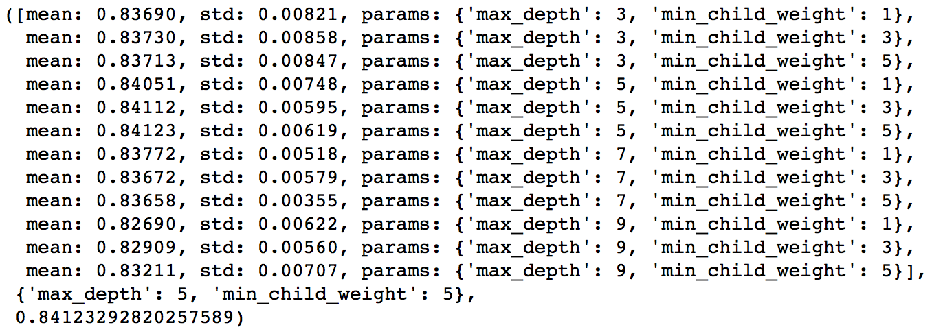
Here, we have run 12 combinations with wider intervals between values. The ideal values are 5 for max_depth and 5 for min_child_weight. Let’s go one step deeper and look for optimum values. We’ll search for values 1 above and below the optimum values because we took an interval of two.
param_test2 = {
 'max_depth':[4,5,6],
 'min_child_weight':[4,5,6]
}
gsearch2 = GridSearchCV(estimator = XGBClassifier( learning_rate=0.1, n_estimators=140, max_depth=5,
 min_child_weight=2, gamma=0, subsample=0.8, colsample_bytree=0.8,
 objective= 'binary:logistic', nthread=4, scale_pos_weight=1,seed=27),
 param_grid = param_test2, scoring='roc_auc',n_jobs=4,iid=False, cv=5)
gsearch2.fit(train[predictors],train[target])
gsearch2.grid_scores_, gsearch2.best_params_, gsearch2.best_score_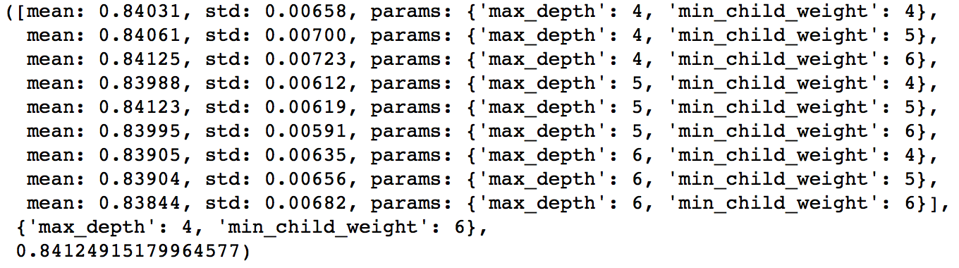
Here, we get the optimum values as 4 for max_depth and 6 for min_child_weight. Also, we can see the CV score increasing slightly. Note that as the model performance increases, it becomes exponentially difficult to achieve even marginal gains in performance. You would have noticed that here we got 6 as the optimum value for min_child_weight, but we haven’t tried values more than 6. We can do that as follow:
param_test2b = {
 'min_child_weight':[6,8,10,12]
}
gsearch2b = GridSearchCV(estimator = XGBClassifier( learning_rate=0.1, n_estimators=140, max_depth=4,
 min_child_weight=2, gamma=0, subsample=0.8, colsample_bytree=0.8,
 objective= 'binary:logistic', nthread=4, scale_pos_weight=1,seed=27),
 param_grid = param_test2b, scoring='roc_auc',n_jobs=4,iid=False, cv=5)
gsearch2b.fit(train[predictors],train[target])
modelfit(gsearch3.best_estimator_, train, predictors)
gsearch2b.grid_scores_, gsearch2b.best_params_, gsearch2b.best_score_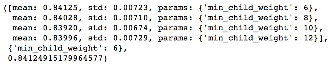
We see 6 as the optimal value.
Step3: Tune gamma
Now let’s tune the gamma value using the parameters already tuned above. Gamma can take various values, but I’ll check for 5 values here. You can go into more precise values.
param_test3 = {
 'gamma':[i/10.0 for i in range(0,5)]
}
gsearch3 = GridSearchCV(estimator = XGBClassifier( learning_rate =0.1, n_estimators=140, max_depth=4,
 min_child_weight=6, gamma=0, subsample=0.8, colsample_bytree=0.8,
 objective= 'binary:logistic', nthread=4, scale_pos_weight=1,seed=27),
 param_grid = param_test3, scoring='roc_auc',n_jobs=4,iid=False, cv=5)
gsearch3.fit(train[predictors],train[target])
gsearch3.grid_scores_, gsearch3.best_params_, gsearch3.best_score_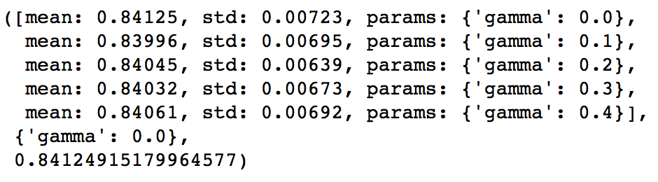
This shows that our original value of gamma, i.e., 0 is the optimum one. Before proceeding, a good idea would be to re-calibrate the number of boosting rounds for the updated parameters.
xgb2 = XGBClassifier(
 learning_rate =0.1,
 n_estimators=1000,
 max_depth=4,
 min_child_weight=6,
 gamma=0,
 subsample=0.8,
 colsample_bytree=0.8,
 objective= 'binary:logistic',
 nthread=4,
 scale_pos_weight=1,
 seed=27)
modelfit(xgb2, train, predictors)
Here, We can see the score improvement. so, the final parameters are:
- max_depth: 4
- min_child_weight: 6
- gamma: 0
Step4: Tune subsample and colsample_bytree
The next step would be to try different subsample and colsample_bytree values. Let’s do this in 2 stages as well and take values 0.6,0.7,0.8,0.9 for both to start with.
param_test4 = {
 'subsample':[i/10.0 for i in range(6,10)],
 'colsample_bytree':[i/10.0 for i in range(6,10)]
}
gsearch4 = GridSearchCV(estimator = XGBClassifier( learning_rate =0.1, n_estimators=177, max_depth=4,
 min_child_weight=6, gamma=0, subsample=0.8, colsample_bytree=0.8,
 objective= 'binary:logistic', nthread=4, scale_pos_weight=1,seed=27),
 param_grid = param_test4, scoring='roc_auc',n_jobs=4,iid=False, cv=5)
gsearch4.fit(train[predictors],train[target])
gsearch4.grid_scores_, gsearch4.best_params_, gsearch4.best_score_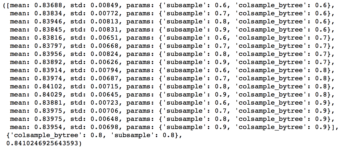
Here, we found 0.8 as the optimum value for both subsample and colsample_bytree. Now we should try values in 0.05 intervals around these.
param_test5 = {
 'subsample':[i/100.0 for i in range(75,90,5)],
 'colsample_bytree':[i/100.0 for i in range(75,90,5)]
}
gsearch5 = GridSearchCV(estimator = XGBClassifier( learning_rate =0.1, n_estimators=177, max_depth=4,
 min_child_weight=6, gamma=0, subsample=0.8, colsample_bytree=0.8,
 objective= 'binary:logistic', nthread=4, scale_pos_weight=1,seed=27),
 param_grid = param_test5, scoring='roc_auc',n_jobs=4,iid=False, cv=5)
gsearch5.fit(train[predictors],train[target])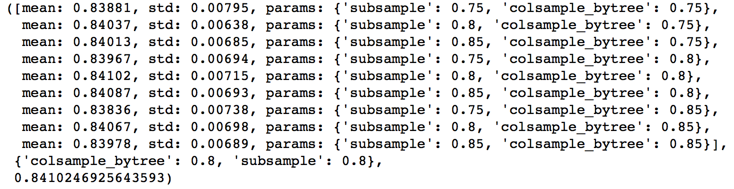
Again we got the same values as before. Thus the optimum values are:
- subsample: 0.8
- colsample_bytree: 0.8
Step5: Tuning Regularization Parameters
The next step is to apply regularization to reduce overfitting. However, many people don’t use this parameter much as gamma provides a substantial way of controlling complexity. But we should always try it. I’ll tune the ‘reg_alpha’ value here and leave it up to you to try different values of ‘reg_lambda’.
param_test6 = {
 'reg_alpha':[1e-5, 1e-2, 0.1, 1, 100]
}
gsearch6 = GridSearchCV(estimator = XGBClassifier( learning_rate =0.1, n_estimators=177, max_depth=4,
 min_child_weight=6, gamma=0.1, subsample=0.8, colsample_bytree=0.8,
 objective= 'binary:logistic', nthread=4, scale_pos_weight=1,seed=27),
 param_grid = param_test6, scoring='roc_auc',n_jobs=4,iid=False, cv=5)
gsearch6.fit(train[predictors],train[target])
gsearch6.grid_scores_, gsearch6.best_params_, gsearch6.best_score_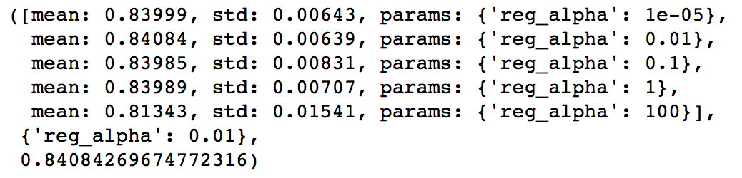
We can see that the CV score is less than in the previous case. But the values tried are very widespread. We should try values closer to the optimum here (0.01) to see if we get something better.
param_test7 = {
 'reg_alpha':[0, 0.001, 0.005, 0.01, 0.05]
}
gsearch7 = GridSearchCV(estimator = XGBClassifier( learning_rate =0.1, n_estimators=177, max_depth=4,
 min_child_weight=6, gamma=0.1, subsample=0.8, colsample_bytree=0.8,
 objective= 'binary:logistic', nthread=4, scale_pos_weight=1,seed=27),
 param_grid = param_test7, scoring='roc_auc',n_jobs=4,iid=False, cv=5)
gsearch7.fit(train[predictors],train[target])
gsearch7.grid_scores_, gsearch7.best_params_, gsearch7.best_score_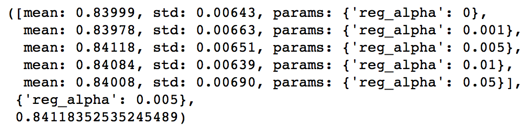
You can see that we got a better CV. Now we can apply this regularization in the model and look at the impact:
xgb3 = XGBClassifier(
 learning_rate =0.1,
 n_estimators=1000,
 max_depth=4,
 min_child_weight=6,
 gamma=0,
 subsample=0.8,
 colsample_bytree=0.8,
 reg_alpha=0.005,
 objective= 'binary:logistic',
 nthread=4,
 scale_pos_weight=1,
 seed=27)
modelfit(xgb3, train, predictors)
Again we can see a slight improvement in the score.
Step6: Reducing the Learning Rate
Lastly, we should lower the learning rate and add more trees. Let’s use the cv function of XGBoost classifier to do the job again.
xgb4 = XGBClassifier(
 learning_rate =0.01,
 n_estimators=5000,
 max_depth=4,
 min_child_weight=6,
 gamma=0,
 subsample=0.8,
 colsample_bytree=0.8,
 reg_alpha=0.005,
 objective= 'binary:logistic',
 nthread=4,
 scale_pos_weight=1,
 seed=27)
modelfit(xgb4, train, predictors)
Here is a live coding window where you can try different parameters and test the results.
import pandas as pd
import numpy as np
import xgboost as xgb
from xgboost.sklearn import XGBClassifier
from sklearn.model_selection import cross_val_score
from sklearn import metrics
from sklearn.model_selection import GridSearchCV

train = pd.read_csv('train_modified_sample.csv')
print(train.head())

print(train['Disbursed'].value_counts())


target='Disbursed'
IDcol = 'ID'

predictors = [x for x in train.columns if x not in [target, IDcol]]

param_test = {
    'reg_alpha':[1e-5, 1e-2, 0.1, 100]
}
gsearch = GridSearchCV(estimator =
XGBClassifier(learning_rate =0.1,
              n_estimators=10,
              max_depth=5,
              min_child_weight=2,
              gamma=0.1,
              subsample=0.85,
              colsample_bytree=0.8,
              objective= 'binary:logistic',
              nthread=4,
              scale_pos_weight=1,
              seed=27),
              param_grid = param_test,
              scoring='roc_auc',
              n_jobs=4,
              iid=False,
              cv=2,
              verbose=10)

gsearch.fit(train[predictors],train[target])

print('Best Grid Search Parameters :',gsearch.best_params_)
print('Best Grid Search Score : ',gsearch.best_score_)
Now we can see a significant boost in performance, and the effect of parameter tuning is clearer.
As we come to an end, I would like to share 2 key thoughts:
- It is difficult to get a very big leap in performance by just using parameter tuning or slightly better models. The max score for GBM was 0.8487, while XGBoost gave 0.8494. This is a decent improvement but not something very substantial.
- A significant jump can be obtained by other methods like feature engineering, creating an ensemble of models, stacking, etc.
You can also download the iPython notebook with all these model codes from my GitHub account. For codes in R, you can refer to this article.
Conclusion
This tutorial was based on developing an XGBoost machine learning model end-to-end. We started by discussing why XGBoost Parameters has superior performance over GBM, which was followed by a detailed discussion of the various parameters involved. We also defined a generic function that you can reuse for making models. Finally, we discussed the general approach towards tackling a problem with XGBoost and also worked out the AV Data Hackathon 3.x problem through that approach.
Hope you like the article! The XGBoost algorithm is a strong tool used in machine learning. The XGBoost classifier helps improve predictions by using an XGBoost model. To understand how XGBoost works, it’s important to know its gradient boosting method, which is explained by how well it manages data.
Key Takeaways
- XGBoost Paramters is a powerful machine-learning algorithm, especially where speed and accuracy are concerned.
- We need to consider different parameters and their values to be specified while implementing an XGBoost model.
- The XGBoost hyperparameters model requires parameter tuning to improve and fully leverage its advantages over other algorithms.
If you’re looking to take your machine learning skills to the next level, consider enrolling in our Data Science Black Belt program. The curriculum covers all aspects of data science, including advanced topics like XGBoost parameter tuning. With hands-on projects and mentorship, you’ll gain practical experience and the skills you need to succeed in this exciting field. Enroll today and take your XGBoost parameters tuning skills and overall data science expertise to the next level!
Frequently Asked Questions
Q1. What parameters should you use for XGBoost?
A. The choice of XGBoost parameters depends on the specific task. Commonly adjusted parameters include learning rate (eta), maximum tree depth (max_depth), and minimum child weight (min_child_weight).
Q2. What does the ‘N_estimators’ parameter signify in XGBoost?
A. The ‘n_estimators’ parameter in XGBoost determines the number of boosting rounds or trees to build. It directly impacts the model’s complexity and should be tuned for optimal performance.
Q3. How do you define a hyperparameter in XGBoost?
A. In XGBoost, a hyperparameter is a preset setting that isn’t learned from the data but must be configured before training. Examples include the learning rate, tree depth, and regularization parameters.
Q4. What purpose do regularization parameters serve in XGBoost?
A. XGBoost provides L1 and L2 regularization terms using the ‘alpha’ and ‘lambda’ parameters, respectively. These parameters prevent overfitting by adding penalty terms to the objective function during training.
Gradient Boostinggrid searchhyperparameter tuning xgboostlive codingparameter tuning in xgboostpythonsklearntuning xgboostxgbclassifier hyperparameter tuningxgbclassifier parametersXGBoostXGBoost classiferxgboost classifierxgboost classifier hyperparameter tuningxgboost classifier parametersxgboost modelxgboost tuningxgbregressor hyperparameter tuningxgbregressor parameters
Aarshay
04 Sep, 2024