Build High Performance Time Series Models using Auto ARIMA in Python and R

Introduction

Picture this – You’ve been tasked with forecasting the price of the next iPhone and have been provided with historical data. This includes features like quarterly sales, month-on-month expenditure, and a whole host of things that come with Apple’s balance sheet. As a data scientist, which kind of problem would you classify this as? Time series modeling, of course.

From predicting the sales of a product to estimating the electricity usage of households, time series forecasting is one of the core skills any data scientist is expected to know, if not master. There are a plethora of different techniques out there which you can use, and we will be covering one of the most effective ones, called Auto ARIMA, in this article.

We will first understand the concept of ARIMA which will lead us to our main topic – Auto ARIMA. To solidify our concepts, we will take up a dataset and implement it in both Python and R.

If you are familiar with time series and it’s techniques (like moving average, exponential smoothing, and ARIMA),  you can skip directly to section 4. For beginners, start from the below section which is a brief introduction to time series and various forecasting techniques.

What is a time series ?

Before we learn about the techniques to work on time series data, we must first understand what a time series actually is and how is it different from any other kind of data. Here is the formal definition of time series – It is a series of data points measured at consistent time intervals. This simply means that particular values are recorded at a constant interval which may be hourly, daily, weekly, every 10 days, and so on. What makes time series different is that each data point in the series is dependent on the previous data points. Let us understand the difference more clearly by taking a couple of examples.

Example 1:

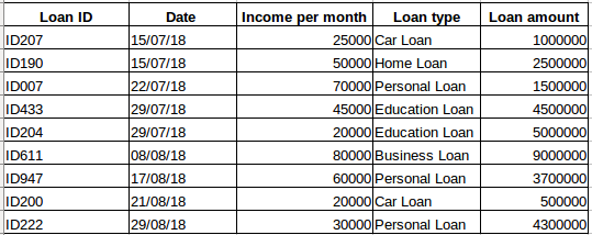
Suppose you have a dataset of people who have taken a loan from a particular company (as shown in the table below). Do you think each row will be related to the previous rows? Certainly not! The loan taken by a person will be based on his financial conditions and needs (there could be other factors such as the family size etc., but for simplicity we are considering only income and loan type) . Also, the data was not collected at any specific time interval. It depends on when the company received a request for the loan.

Example 2:

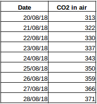
Let’s take another example. Suppose you have a dataset that contains the level of CO2 in the air per day (screenshot below). Will you be able to predict the approximate amount of CO2 for the next day by looking at the values from the past few days? Well, of course. If you observe, the data has been recorded on a daily basis, that is, the time interval is constant (24 hours).

You must have got an intuition about this by now – the first case is a simple regression problem and the second is a time series problem. Although the time series puzzle here can also be solved using linear regression, but that isn’t really the best approach as it neglects the relation of the values with all the relative past values. Let’s now look at some of the common techniques used for solving time series problems.

Methods for time series forecasting

There are a number of methods for time series forecasting and we will briefly cover them in this section. The detailed explanation and python codes for all the below mentioned techniques can be found in this article: 7 techniques for time series forecasting (with python codes).

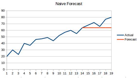
1. Naive Approach: In this forecasting technique, the value of the new data point is predicted to be equal to the previous data point. The result would be a flat line, since all new values take the previous values.
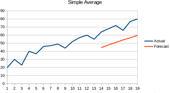
2. Simple Average: The next value is taken as the average of all the previous values. The predictions here are better than the ‘Naive Approach’ as it doesn’t result in a flat line but here, all the past values are taken into consideration which might not always be useful. For instance, when asked to predict today’s temperature, you would consider the last 7 days’ temperature rather than the temperature a month ago.
3. Moving Average : This is an improvement over the previous technique. Instead of taking the average of all the previous points, the average of ‘n’ previous points is taken to be the predicted value.
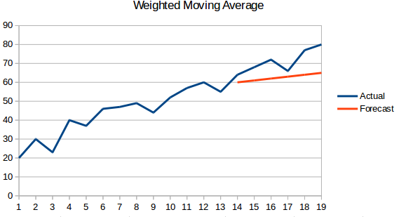
4. Weighted moving average : A weighted moving average is a moving average where the past ‘n’ values are given different weights.
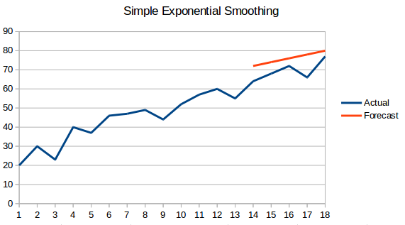
5. Simple Exponential Smoothing: In this technique, larger weights are assigned to more recent observations than to observations from the distant past.
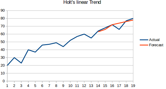
6. Holt’s Linear Trend Model: This method takes into account the trend of the dataset. By trend, we mean the increasing or decreasing nature of the series. Suppose the number of bookings in a hotel increases every year, then we can say that the number of bookings show an increasing trend. The forecast function in this method is a function of level and trend.
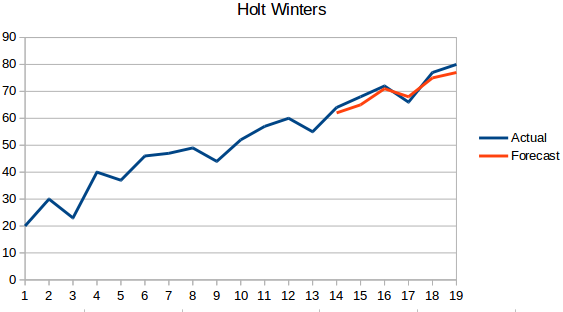
7. Holt Winters Method: This algorithm takes into account both the trend and the seasonality of the series. For instance – the number of bookings in a hotel is high on weekends & low on weekdays, and increases every year; there exists a weekly seasonality and an increasing trend.
8. ARIMA: ARIMA is a very popular technique for time series modeling. It describes the correlation between data points and takes into account the difference of the values. An improvement over ARIMA is SARIMA (or seasonal ARIMA). We will look at ARIMA in a bit more detail in the following section.

Introduction to ARIMA

In this section we will do a quick introduction to ARIMA which will be helpful in understanding Auto Arima. A detailed explanation of Arima, parameters (p,q,d), plots (ACF PACF) and implementation is included in this article : Complete tutorial to Time Series.

ARIMA is a very popular statistical method for time series forecasting. ARIMA stands for Auto-Regressive Integrated Moving Averages. ARIMA models work on the following assumptions –

• The data series is stationary, which means that the mean and variance should not vary with time. A series can be made stationary by using log transformation or differencing the series.
• The data provided as input must be a univariate series, since arima uses the past values to predict the future values.

ARIMA has three components – AR (autoregressive term), I (differencing term) and MA (moving average term). Let us understand each of these components –

• AR term refers to the past values used for forecasting the next value. The AR term is defined by the parameter ‘p’ in arima. The value of ‘p’ is determined using the PACF plot.
• MA term is used to defines number of past forecast errors used to predict the future values. The parameter ‘q’ in arima represents the MA term. ACF plot is used to identify the correct ‘q’ value.
• Order of differencing  specifies the number of times the differencing operation is performed on series to make it stationary. Test like ADF and KPSS can be used to determine whether the series is stationary and help in identifying the d value.

Steps for ARIMA implementation

What is Auto ARIMA?

Auto ARIMA (Auto-Regressive Integrated Moving Average) is a statistical algorithm used for time series forecasting. It automatically determines the optimal parameters for an ARIMA model, such as the order of differencing, autoregressive (AR) terms, and moving average (MA) terms. Auto ARIMA searches through different combinations of these parameters to find the best fit for the given time series data. This automated process saves time and effort, making it easier for users to generate accurate forecasts without requiring extensive knowledge of time series analysis.

Why do we need Auto ARIMA?

Although ARIMA is a very powerful model for forecasting time series data, the data preparation and parameter tuning processes end up being really time consuming. Before implementing ARIMA, you need to make the series stationary, and determine the values of p and q using the plots we discussed above. Auto ARIMA makes this task really simple for us as it eliminates steps 3 to 6 we saw in the previous section. Below are the steps you should follow for implementing auto ARIMA:

1. Load the data: This step will be the same. Load the data into your notebook
2. Preprocessing data: The input should be univariate, hence drop the other columns
3. Fit Auto ARIMA: Fit the model on the univariate series
4. Predict values on validation set: Make predictions on the validation set
5. Calculate RMSE: Check the performance of the model using the predicted values against the actual values

We completely bypassed the selection of p and q feature as you can see. What a relief! In the next section, we will implement auto ARIMA using a toy dataset.

Implementation in Python and R

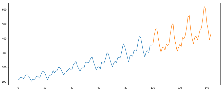
We will be using the International-Air-Passenger dataset. This dataset contains monthly total of number of passengers (in thousands). It has two columns – month and count of passengers. You can download the dataset from this link.
Python Code:

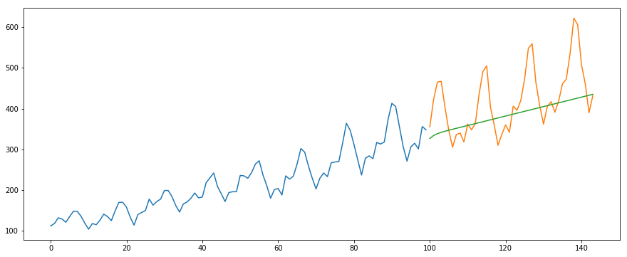
#building the model
from pyramid.arima import auto_arima
model = auto_arima(train, trace=True, error_action='ignore', suppress_warnings=True)
model.fit(train)

forecast = model.predict(n_periods=len(valid))
forecast = pd.DataFrame(forecast,index = valid.index,columns=['Prediction'])

#plot the predictions for validation set
plt.plot(train, label='Train')
plt.plot(valid, label='Valid')
plt.plot(forecast, label='Prediction')
plt.show()

#calculate rmse
from math import sqrt
from sklearn.metrics import mean_squared_error

rms = sqrt(mean_squared_error(valid,forecast))
print(rms)

output -
76.51355764316357

Below is the R Code for the same problem:

# loading packages
library(forecast)
library(Metrics)

# reading data
data = read.csv("international-airline-passengers.csv")

# splitting data into train and valid sets
train = data[1:100,]
valid = data[101:nrow(data),]

# removing "Month" column
train$Month = NULL

# training model
model = auto.arima(train)

# model summary
summary(model)

# forecasting
forecast = predict(model,44)

# evaluation
rmse(valid$International.airline.passengers, forecast$pred)

How does Auto Arima select the best parameters

In the above code, we simply used the .fit() command to fit the model without having to select the combination of p, q, d. But how did the model figure out the best combination of these parameters? Auto ARIMA takes into account the AIC and BIC values generated (as you can see in the code) to determine the best combination of parameters. AIC (Akaike Information Criterion) and BIC (Bayesian Information Criterion) values are estimators to compare models. The lower these values, the better is the model.

Check out these links if you are interested in the maths behind AIC and BIC.

Frequently Asked Questions

End Notes and Further Reads

I have found auto ARIMA to be the simplest technique for performing time series forecasting. Knowing a shortcut is good but being familiar with the math behind it is also important. In this article I have skimmed through the details of how ARIMA works but do make sure that you go through the links provided in the article. For your easy reference, here are the links again:

• A Comprehensive Guide for beginners to Time Series Forecast in Python
• Complete Tutorial to Time series in R
• 7 techniques for time series forecasting (with python codes)

I would suggest practicing what we have learned here on this practice problem: Time Series Practice Problem. You can also take our training course created on the same practice problem, Time series forecasting, to provide you a head start.

Good luck, and feel free to provide your feedback and ask questions in the comments section below.

AishwaryaSingh 23 May, 2023