Create a Dummy Stock Market Using Geometric Brownian Motion in Python

Introduction :

The goal is to create a replica of a financial stock market or this can be extended to the cryptocurrency market also using Geometric Brownian Motion.

Source

Stochastic processes are full of options and anyone who wants to begin trading can first experiment on a demo market and strategies accordingly as to how the market plays out when the variables change. You can simulate a market and change your strategy and plan it out accordingly and decide the final one for you.

ROI ( Return on Investment)

Source

The most important factor in the stock market is the returns on any share. If we consider the price of a particular day ‘n’ and let the previous day be denoted by ‘n-1’. Then the returns can be calculated by the formula :

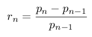
Then using this formula we can create a price time series by using the following formula :

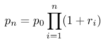
So if we know the first starting price or p₀ then we can calculate the future price of the stock using the sequence of returns.

The one thing about the model is that all the returns are stochastic objects and hence all the different realization of the various returns will give us a different time series for all the prices. The behavior of the price is modeled in this way.

Hence to prepare our model, we need to assume a few parameters about the returns and then apply the above formula. The one formula we will be using here which is the Geometric Brownian Motion is one of these assumptions.

What is Geometric Brownian Motion?

Source

The Geometric Brownian Motion is a specific model for the stock market where the returns are not correlated and distributed normally. It can be mathematically written as :

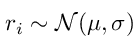
This means that the returns are normally distributed with a mean of ‘μ‘ and the standard deviation is denoted by ‘σ‘. We need to keep in mind that their parameters are all-time dependant and hence these processes are known as stationary.

μ: This symbol denotes the mean value of the returns. A positive value denotes a bullish trend and a negative value denotes a bearish trend. The higher the absolute value of this parameter, the stronger the trend.

σ: This symbol denotes the volatility of the returns and a higher value denotes a more erratic price.

Overall you can analyze your portfolio with the Sharpe Ratio with a risk-free return equals to 0 and can be denoted by ‘μ/σ’. If you love the maths behind the statistics, you can move on a continuous-time and we can use an SDE or Stochastic Differential Equation.

For those of you who, like me, love the math behind statistics, if we switch to a continuous time we can write this stochastic differential equation (SDE):

dr_t =   μr_tdt + σr_tdW_t

where W denotes the ‘Wiener process’

This model is also used in financial mathematics because it is one of the simplest stock market simulations which can be built. This is also the theoretical base of the Nobel Aware Black Sholes options theory. Though while applying with the real market, we need to consider other factors into the equation and remember that the stock market returns are not normally distributed and neither stationary. Though it is a good starting point to begin from.

The idea is that we generate n normally distributed random variables and then calculate the future prices after starting from a start price. We can achieve this in less than 10 lines of code in Python.

Python Code

Source

We will begin  by importing some useful libraries with their usual naming conventions :

import numpy as np
import matplotlib.pyplot as plt

Now we will define the following parameters, to begin with, which can be changed later to test out different outcomes and how each of the variables can influence the end result.

mu = 0.001
sigma = 0.01
start_price = 5

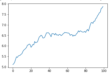
Now coming to the simulation part, we need to set a seed for NumPy random number generator so that we can make reproducible results. We create 100 values for returns and then we build the time series beginning from the starting price.

np.random.seed(0)
returns = np.random.normal(loc=mu, scale=sigma, size=100)
price = start_price*(1+returns).cumprod()

You can more values for a more detailed one or even less, that is entirely up to you, and then finally, we will plot out results :

That is all and we did it in 9 lines of code only.

We can change various parameters and see how it affects the stock market. For example, if we change the value of ‘μ’ and then inspect the results :

If we change the value of μ to 0.004, we get the following graph :

Hence we can conclude that a higher value of ‘μ’ will lead to a stronger and bullish trend.

Similarly, if we increase the value of the other parameter we will find more interesting results about how volatility affects a stock in the long term and this will help you decide how much you want to invest in safe stocks and how much into volatile ones. Whatever be the ultimate result, you should never put all your eggs in one basket and hence always diversify your portfolio. The information in this article is for educational purposes only and should not be taken as financial advice. The author or the platform is in no way responsible for your financial actions.

Conclusions 

Creating a Stock market in python using the GBM is easy to do but then we need to remember that the stock market is not always normally distributed and hence we can apply a time dependence factor on ‘μ’ and ‘σ’. We can also use a separate probability distribution function for the returns and achieve a better result. Replicating the same results for multiple stocks over a certain amount of time and with variable return parameters can actually replicate a whole stock market with different stocks. In the real world, the most important factor to consider is that the ROI or return on investment is not continuous but it is a discrete function.

The link to an online google collab notebook can be found here.

Arnab Mondal 19 Sep 2022

Just a guy who loves to code and learn new languages and concepts