This article explains the problem of exploding and vanishing gradients while training a deep neural network and the techniques that can be used to cleverly get past this impediment.In this article, you will get a clarify about vanishing and exploding gradients and their problem and solutions with that you will get to know about exploding agents and vanishing agents what they are and how their problem is solved in this article. So let’s begin.
This article was published as a part of the Data Science Blogathon
We know that the backpropagation algorithm is the heart of neural network training. Let’s have a glimpse over this algorithm that has proved to be a harbinger in the evolution as well as the revolution of Deep Learning.
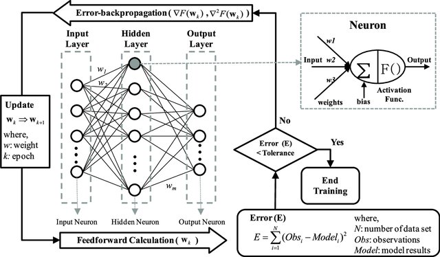
After propagating the input features forward to the output layer through the various hidden layers consisting of different/same activation functions, we come up with a predicted probability of a sample belonging to the positive class ( generally, for classification tasks).
As the backpropagation algorithm advances downwards(or backward) from the output layer towards the input layer, the gradients often get smaller and smaller and approach zero which eventually leaves the weights of the initial or lower layers nearly unchanged. As a result, the gradient descent never converges to the optimum. This is known as the vanishing gradients problem.
On the contrary, in some cases, the gradients keep on getting larger and larger as the backpropagation algorithm progresses. This, in turn, causes very large weight updates and causes the gradient descent to diverge. This is known as the exploding gradients problems.
Certain activation functions, like the logistic function (sigmoid), have a very huge difference between the variance of their inputs and the outputs. In simpler words, they shrink and transform a larger input space into a smaller output space that lies between the range of [0,1].
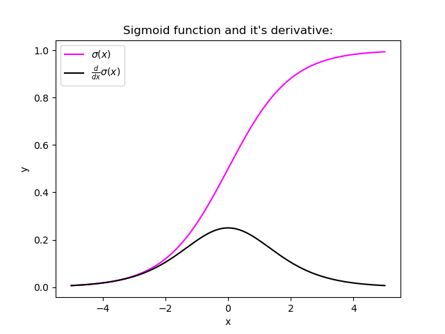
Observing the above graph of the Sigmoid function, we can see that for larger inputs (negative or positive), it saturates at 0 or 1 with a derivative very close to zero. Thus, when the backpropagation algorithm chips in, it virtually has no gradients to propagate backward in the network, and whatever little residual gradients exist keeps on diluting as the algorithm progresses down through the top layers. So, this leaves nothing for the lower layers.
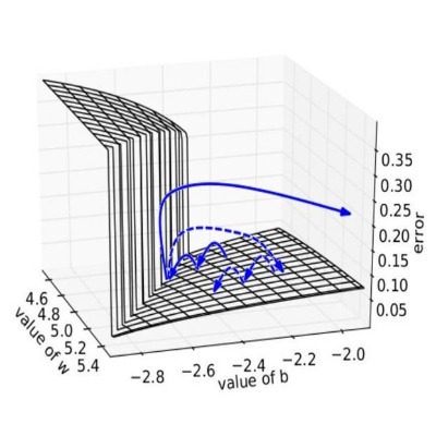
Similarly, in some cases suppose the initial weights assigned to the network generate some large loss. Now the gradients can accumulate during an update and result in very large gradients which eventually results in large updates to the network weights and leads to an unstable network. The parameters can sometimes become so large that they overflow and result in NaN values.
Following are some signs that can indicate that our gradients are vanishing and exploding gradients :
| Exploding | Vanishing | |
| There is an exponential growth in the model parameters. | The parameters of the higher layers change significantly whereas the parameters of lower layers would not change much (or not at all). | |
| The model weights may become NaN during training. | The model weights may become 0 during training. |
| The model experiences avalanche learning. | The model learns very slowly and perhaps the training stagnates at a very early stage just after a few iterations. | |
Certainly, neither do we want our signal to explode or saturate nor do we want it to die out. The signal needs to flow properly both in the forward direction when making predictions as well as in the backward direction while calculating gradients.
Now that we understand the vanishing/exploding gradients problems, we can learn some techniques to fix them.
In their paper, researchers Xavier Glorot, Antoine Bordes, and Yoshua Bengio proposed a way to remarkably alleviate this problem.
For the proper flow of the signal, the authors argue that:
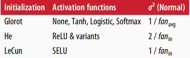
Although both conditions cannot hold for any layer in the network unless the number of inputs to the layer (fanin) equals the number of neurons in the layer (fanout), they proposed a well-proven compromise that works incredibly well in practice. They randomly initialize the connection weights for each layer in the network using the following equation, popularly known as Xavier initialization (after the author’s first name) or Glorot initialization (after his last name).
where fanavg = ( fanin + fanout ) / 2Following are some more very popular weight initialization strategies for different activation functions, they only differ by the scale of variance and by the usage of either fanavg or fanin
for uniform distribution, calculate r as: r = sqrt( 3*σ2 )
Using the above initialization strategies can significantly speed up the training and increase the odds of gradient descent converging at a lower generalization error.
Relax! we will not need to hardcode anything, Keras does it for us.
keras.layer.Dense(25, activation = "relu", kernel_initializer="he_normal")or
keras.layer.Dense(25, activation = "relu", kernel_initializer="he_uniform")If we wish to use use the initialization based on fanavg rather than fanin , we can use the VarianceScaling initializer like this :
he_avg_init = keras.initializers.VarianceScaling(scale=2., mode='fan_avg', distribution='uniform')
keras.layers.Dense(20, activation="sigmoid", kernel_initializer=he_avg_init)In an earlier section, while studying the nature of sigmoid activation function, we observed that its nature of saturating for larger inputs (negative or positive) came out to be a major reason behind the vanishing and exploding gradients thus making it non-recommendable to use in the hidden layers of the network.
So to tackle the issue regarding the saturation of activation functions like sigmoid and tanh, we must use some other non-saturating functions like ReLu and its alternatives.
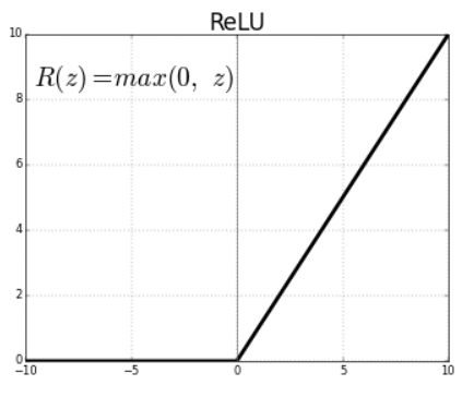
Relu(z) = max(0,z)Unfortunately, the ReLu function is also not a perfect pick for the intermediate layers of the network “in some cases”. It suffers from a problem known as dying ReLus wherein some neurons just die out, meaning they keep on throwing 0 as outputs with the advancement in training.
Read about the dying relus problem in detail here.
Some popular alternative functions of the ReLU that mitigates the problem of vanishing gradients when used as activation for the intermediate layers of the network are LReLU, PReLU, ELU, SELU :
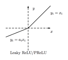
LeakyReLUα(z) = max(αz, z).png)
For z < 0, it takes on negative values which allow the unit to have an average output closer to 0 thus alleviating the vanishing gradient problem
Using He initialization along with any variant of the ReLU activation function can significantly reduce the chances of vanishing/exploding problems at the beginning. However, it does not guarantee that the problem won’t reappear during training.
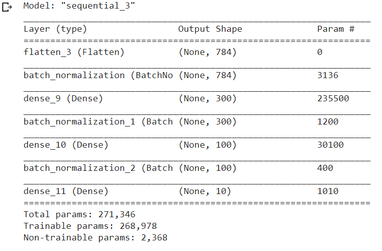
In 2015, Sergey Ioffe and Christian Szegedy proposed a paper in which they introduced a technique known as Batch Normalization to address the problem of vanishing/exploding gradient problem.
The Following key points explain the intuition behind BN and how it works:
model = keras.models.Sequential([keras.layers.Flatten(input_shape=[28, 28]),keras.layers.BatchNormalization(),keras.layers.Dense(300, activation="relu"),keras.layers.BatchNormalization(),keras.layers.Dense(100, activation="relu"),keras.layers.BatchNormalization(),keras.layers.Dense(10, activation="softmax")])we just added batch normalization after each layer ( dataset : FMNIST)model.summary()
Another popular technique to mitigate the exploding gradient problem is to clip the gradients during backpropagation so that they never exceed some threshold. This is called Gradient Clipping.
optimizer = keras.optimizers.SGD(clipvalue = 1.0)optimizer = keras.optimizers.SGD(clipnorm = 1.0)I hope the article would have helped you understand the problem of exploding/vanishing gradients thoroughly and you will be able to identify if by any chance your model suffers from it and you can easily tackle it and train your model efficiently.
Thanks for your time. HAPPY LEARNING
The media shown in this article are not owned by Analytics Vidhya and are used at the Author’s discretion.
A. Exploding gradients occur when model gradients grow uncontrollably during training, causing instability. Vanishing gradients happen when gradients shrink excessively, hindering effective learning and updates.
A. The vanishing gradient problem refers to the phenomenon where gradients diminish as they are propagated backward through layers, making it difficult for models to learn and update weights, especially in deep networks.
A. In RNNs, the vanishing gradient problem impedes learning long-term dependencies due to diminishing gradients, while the exploding gradient problem causes instability and divergent updates due to excessively large gradients.
A. An exploding gradient plot visualizes the sudden increase in gradient values during training, indicating instability and potential divergence, often requiring gradient clipping or other techniques to mitigate the issue.
Lorem ipsum dolor sit amet, consectetur adipiscing elit,


