Machine learning projects work best when they connect theory to real business outcomes. In e-commerce, that means better revenue, smoother operations, and happier customers, all driven by data. By working with realistic datasets, practitioners learn how models turn patterns into decisions that actually matter.
This article walks through a full machine learning workflow using an Amazon sales dataset, from problem framing to a submission ready prediction file. It gives learners a clear view of how models turn insights into business value, in this article.
Table of contents
- Understanding the problem statement
- About the dataset
- Load essential Python Libraries
- Load the datasets
- Data Preprocessing
- Exploratory data analysis (EDA)
- Feature Engineering
- Splitting the train and test data
- Build Machine Learning Model
- Make predictions on the test dataset
- Prepare submission file
- Conclusion
- Frequently Asked Questions
Understanding the problem statement
Before proceeding with the coding part, it is essential to look up to the problem statement and understand it. The dataset consists of Amazon e-commerce transactions which show authentic online shopping patterns from actual online retail activities.
The primary objective of this project is to predict order outcomes and analyze revenue-driving factors using structured transactional data. The development process requires us to create a supervised machine learning model which learns from past transaction data to forecast results on new test datasets.
Key Business Questions Addressed
- Which factors influence the final order amount?
- How do discounts, taxes, and shipping costs affect revenue?
- Can we predict order status or total transaction value accurately?
- What insights can businesses extract to improve sales performance?
About the dataset
The dataset consists of 100,000 e-commerce transactions which follow Amazon’s transaction style and include 20 organized data fields. The synthetic data exhibits authentic customer behavior patterns together with actual business operation processes.
The data set contains information about price changes across different product types and customer age groups and their payment options and their order tracking statuses. The data set contains properties which make it suitable for machine learning and analytical work and dashboard development.
| Section | Field Name |
|---|---|
| Order Details | OrderID |
| OrderDate | |
| OrderStatus | |
| SellerID | |
| Customer Information | CustomerID |
| CustomerName | |
| City | |
| State | |
| Country | |
| Product Information | ProductID |
| ProductName | |
| Category | |
| Brand | |
| Quantity | |
| Pricing & Revenue Metrics | UnitPrice |
| Discount | |
| Tax | |
| ShippingCost | |
| TotalAmount | |
| Payment Details | PaymentMethod |
Load essential Python Libraries
To work on the model development process first it requires essential Python library imports to handle data work. The combination of Pandas and NumPy will enable us to perform both data handling tasks and mathematical calculations. Our visualization needs will be fulfilled through the use of Matplotlib and Seaborn. Scikit-learn provides functions for preprocessing and ML algorithms. Here is the typical set of imports:
import pandas as pd
import numpy as np
import matplotlib.pyplot as plt
import seaborn as sns
from sklearn.model_selection import train_test_split
from sklearn.preprocessing import LabelEncoder
from sklearn.ensemble import RandomForestClassifier
from sklearn.metrics import classification_report, accuracy_score
The libraries enable us to perform four main activities which include loading CSV data, executing data cleansing and transformation processes, using charts for trend analysis, and building a classification model.
Load the datasets
We will import data into a Pandas dataFrame after we complete our environment setup. The raw CSV file undergoes transformation through this step into an analyzable and programmatically manipulatable format.
df = pd.read_csv("Amazon.csv")

print("Shape:", df.shape)
Shape: (100000, 20)
We need to check the data structure after loading because we need confirmation that it was imported correctly. The dataset dimensions are checked while we search for any initial problems that affect data quality.
print("\nMissing values:\n", df.isna().sum())

df.head()
Missing values:
OrderID 0
OrderDate 0
CustomerID 0
CustomerName 0
ProductID 0
ProductName 0
Category 0
Brand 0
Quantity 0
UnitPrice 0
Discount 0
Tax 0
ShippingCost 0
TotalAmount 0
PaymentMethod 0
OrderStatus 0
City 0
State 0
Country 0
SellerID 0
dtype: int64
| OrderID | OrderDate | CustomerID | CustomerName | ProductID | ProductName | Category | Brand | Quantity | UnitPrice | Discount | Tax | ShippingCost | TotalAmount | PaymentMethod | OrderStatus | City | State | Country | SellerID |
|---|---|---|---|---|---|---|---|---|---|---|---|---|---|---|---|---|---|---|---|
| ORD0000001 | 2023-01-31 | CUST001504 | Vihaan Sharma | P00014 | Drone Mini | Books | BrightLux | 3 | 106.59 | 0.00 | 0.00 | 0.09 | 319.86 | Debit Card | Delivered | Washington | DC | India | SELL01967 |
| ORD0000002 | 2023-12-30 | CUST000178 | Pooja Kumar | P00040 | Microphone | Home & Kitchen | UrbanStyle | 1 | 251.37 | 0.05 | 19.10 | 1.74 | 259.64 | Amazon Pay | Delivered | Fort Worth | TX | United States | SELL01298 |
| ORD0000003 | 2022-05-10 | CUST047516 | Sneha Singh | P00044 | Power Bank 20000mAh | Clothing | UrbanStyle | 3 | 35.03 | 0.10 | 7.57 | 5.91 | 108.06 | Debit Card | Delivered | Austin | TX | United States | SELL00908 |
| ORD0000004 | 2023-07-18 | CUST030059 | Vihaan Reddy | P00041 | Webcam Full HD | Home & Kitchen | Zenith | 5 | 33.58 | 0.15 | 11.42 | 5.53 | 159.66 | Cash on Delivery | Delivered | Charlotte | NC | India | SELL01164 |
Data Preprocessing
1. Decomposing Date Features
Models cannot do math on a string like “2023-01-31”. The two elements “Month: 1” and “Year: 2023” create essential numerical attributes which can detect seasonal patterns including holiday sales.
df["OrderDate"] = pd.to_datetime(df["OrderDate"], errors="coerce")
df["OrderYear"] = df["OrderDate"].dt.year
df["OrderMonth"] = df["OrderDate"].dt.month
df["OrderDay"] = df["OrderDate"].dt.day
We have successfully extracted three new features: OrderYear, OrderMonth, and OrderDay. The model learns patterns which show “December brings higher sales” and “weekend days produce increased sales”.
2. Dropping Irrelevant Features
The model requires only specific columns. The unique ID identifiers (OrderID, CustomerID) do not provide predictive information which leads to model training data memorization through overfitting. We also dropped OrderDate since we just extracted its useful parts.
cols_to_drop = [
   "OrderID",
   "CustomerID",
   "CustomerName",
   "ProductID",
   "ProductName",
   "SellerID",
   "OrderDate",   # already decomposed
]

df = df.drop(columns=cols_to_drop)
The dataframe now contains only essential elements which create predictive value. The model now detects common patterns through product category and tax rates while we remove specific customer ID information which could create “leakage” and noise.
3. Handling Missing Values
The initial check showed no missing values but we need our systems to handle real-world conditions. The model will crash if upcoming data contains missing information. We implement a safety net by filling gaps with the median (for numbers) or “Unknown” (for text).
print("\nMissing values after transformations:\n", df.isna().sum())

# If any missing values in numeric columns, fill with median
numeric_cols = df.select_dtypes(include=["int64", "float64"]).columns.tolist()

for col in numeric_cols:
    if df[col].isna().sum() > 0:
        df[col] = df[col].fillna(df[col].median())
Category 0
Brand 0
Quantity 0
UnitPrice 0
Discount 0
Tax 0
ShippingCost 0
TotalAmount 0
PaymentMethod 0
OrderStatus 0
City 0
State 0
Country 0
OrderYear 0
OrderMonth 0
OrderDay 0
dtype: int64
# For categorical columns, fill with "Unknown"
categorical_cols = df.select_dtypes(include=["object"]).columns.tolist()

for col in categorical_cols:
    df[col] = df[col].fillna("Unknown")

print("\nFinal dtypes after cleaning:\n")
Category object
Brand object
Quantity int64
UnitPrice float64
Discount float64
Tax float64
ShippingCost float64
TotalAmount float64
PaymentMethod object
OrderStatus object
City object
State object
Country object
OrderYear int32
OrderMonth int32
OrderDay int32
dtype: object
The pipeline is now bulletproof. The final dtypes check confirms that our data is fully prepped: all categorical variables are objects (ready for encoding) and all numerical variables are int32 or float64 (ready for scaling).
Exploratory data analysis (EDA)
The Data Analysis process begins with our preliminary examination of data which we treat as an interview process to learn about the data’s characteristics. Our investigation includes three main elements which we use to identify patterns and outliers and examine distributional characteristics.
Statistical Summary: We need to understand the mathematical properties of our numerical columns. Are the prices reasonable? Are there any negative values that exist in prohibited areas?
# 2. Basic Data Understanding / EDA (lightweight)
print("\nDescriptive stats (numeric):\n")

df.describe()
The descriptive statistics table provides critical context:
- Quantity: The measurement goes from 1 to 5 with three as its average value. Consumers who shop at retail stores tend to show this behavior which businesses use for their B2B purchases.
- UnitPrice: The price ranges between 5.00 and 599.99 which shows that there exists multiple product tiers.
The target variable TotalAmount shows wide variance because its standard deviation approaches 724 which means our model must maintain its capacity to process transactions ranging from small purchases to maximum purchases of 3534.98.
Categorical Analysis
We need to know the cardinality (number of unique values) of our categorical features. The model experiences bloat and overfitting issues because high cardinality occurs when there are thousands of unique cities in the dataset.
print("\nUnique values in some categorical columns:")

for col in ["Category", "Brand", "PaymentMethod", "OrderStatus", "Country"]:
    print(f"{col}: {df[col].nunique()} unique")
Unique values in some categorical columns:
Category: 6 unique
Brand: 10 unique
PaymentMethod: 6 unique
OrderStatus: 5 unique
Country: 5 unique
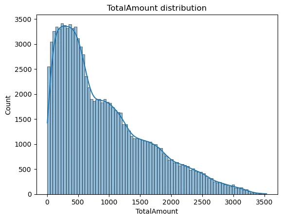
Visualizing the Target Distribution
The histogram shows the frequency of different transaction amounts. A smooth curve (KDE) allows us to see the density. With the curve being slightly right skewed therefore tree-based models like Random Forest handle very well.
sns.histplot(df["TotalAmount"], kde=True)
plt.title("TotalAmount distribution")
plt.show()
The TotalAmount visualization enables us to determine whether the data exhibits any skewed distribution. The data requires a Log Transformation when it shows extreme skewness with only a few high-priced products and numerous low-cost items.
Feature Engineering
Feature engineering develops new variables through the process of transforming existing variables to boost model performance. In Supervised Learning, we must explicitly tell the model what to predict (y) and what data to use to make that prediction (X).
target_column = "TotalAmount"

X = df.drop(columns=[target_column])
y = df[target_column]

numeric_features = X.select_dtypes(include=["int64", "float64"]).columns.tolist()
categorical_features = X.select_dtypes(include=["object"]).columns.tolist()

print("\nNumeric features:", numeric_features)
print("Categorical features:", categorical_features)
Splitting the train and test data
The model evaluation process requires separate data because training data cannot be used for assessment, which parallels the practice of providing students with exam answers before the test. The data distribution consists of two parts: Training Set which serves educational purposes and Test Set which verifies results.
X_train, X_test, y_train, y_test = train_test_split(
    X, y, test_size=0.2, random_state=42
)

print("\nTrain shape:", X_train.shape, "Test shape:", X_test.shape)
Here we have used the 80-20 percent rule, which means randomly out of all the data we have 80% will be used as the train data and the rest 20% will be used to test it as the test data set.
Build Machine Learning Model
Creating the ML pipeline would involved the following processes:
1. Creating Preprocessing Pipelines
The raw numbers of each measurement scale differently because they include measurements that range from 1 to 5 for Quantity and from 5 to 500 for Price. The models achieve faster convergence when researchers implement data scaling techniques. One-Hot Encoding provides the necessary method to transform categorical text into numerical format. The ColumnTransformer system enables us to apply different transformation methods for every column type in our dataset.
numeric_transformer = Pipeline(
    steps=[
        ("scaler", StandardScaler())
    ]
)

categorical_transformer = Pipeline(
    steps=[
        ("onehot", OneHotEncoder(handle_unknown="ignore"))
    ]
)

preprocessor = ColumnTransformer(
    transformers=[
        ("num", numeric_transformer, numeric_features),
        ("cat", categorical_transformer, categorical_features),
    ]
)
2. Defining the Random Forest Model
We have selected the Random Forest Regressor for this project. The ensemble method constructs multiple decision trees which it uses to compute forecast results through prediction averaging. The system demonstrates strong robustness against overfitting problems while it excels at managing non-linear connections between variables.
model = RandomForestRegressor(
    n_estimators=200,
    max_depth=None,
    random_state=42,
    n_jobs=-1
)

# Full pipeline
regressor = Pipeline(
    steps=[
        ("preprocessor", preprocessor),
        ("model", model),
    ]
)
We created the model with n_estimators=200 to build 200 decision trees and n_jobs=-1 to enable all CPU cores for speedier model development. The best practice for this implementation requires users to create a single Pipeline object which combines the preprocessor and model to handle their entire operational process as one unit.
3. Training the Model
This stage represents the primary learning process. The pipeline processes training data through transformation steps before it uses the Random Forest model on the converted data.
regressor.fit(X_train, y_train)

print("\nModel training complete.")
The model now understands how different input variables (Category Price Tax etc.) relate to the output variable (Total Amount).
Make predictions on the test dataset
Now we test the model on the test data (i.e, 20,000 “unseen” records). The model performance assessment uses statistical metrics to compare its predicted outcomes (y_pred) with the actual results (y_test).
y_pred = regressor.predict(X_test)

mae = mean_absolute_error(y_test, y_pred)
mse = mean_squared_error(y_test, y_pred)
rmse = np.sqrt(mse)
r2 = r2_score(y_test, y_pred)

print("\nTest metrics:")
print("MAE :", mae)
print("MSE :", mse)
print("RMSE:", rmse)
print("R2  :", r2)
Test metrics:
MAE : 3.886121525000014
MSE : 41.06268576375389
RMSE: 6.408017303640331
R2 : 0.99992116450905
This signifies:
- The Mean Absolute Error (MAE) value stands at approximately 3.88. Our prediction shows an average error of $3.88.
- The R2 Score value stands at approximately 0.9999. This is near perfect. The independent variables (Price, Tax, Shipping) almost entirely account for the Total Amount according to this result. The Total formula in synthetic financial data follows the equation Total = Price * Qty + Tax + Shipping – Discount.
Prepare submission file
The system requires participants to present their predictions according to predetermined output specifications which must not be altered.
submission = pd.DataFrame({
   "OrderID": df.loc[X_test.index, "OrderID"],
   "PredictedTotalAmount": y_pred
})

submission.to_csv("submission.csv", index=False)
The evaluation system accepts this file for direct submission while stakeholders can also receive it.
Conclusion
This machine learning project demonstrates its complete process through demonstration of raw e-commerce transaction data transformation into useful predictive results. The structured workflow method enables you to manage actual datasets with complete assurance and understanding of the process. The success of the project depends on the five steps which include preprocessing and EDA and feature engineering and modeling.
The project helps in developing your machine learning capabilities while training you to handle real work situations. The pipeline needs additional optimization work before it can function as a recommendation system with advanced models or deep learning techniques.
Frequently Asked Questions
Q1. What is the main goal of this Amazon sales machine learning project?
A. It aims to predict the total order amount using transactional and pricing data.
Q2. Why was a Random Forest model chosen for this project?
A. It captures complex patterns and reduces overfitting by combining many decision trees.
Q3. What does the final submission file contain?
A. It includes OrderID and the model’s predicted total amount for each order.
Hello! I'm Vipin, a passionate data science and machine learning enthusiast with a strong foundation in data analysis, machine learning algorithms, and programming. I have hands-on experience in building models, managing messy data, and solving real-world problems. My goal is to apply data-driven insights to create practical solutions that drive results. I'm eager to contribute my skills in a collaborative environment while continuing to learn and grow in the fields of Data Science, Machine Learning, and NLP.


