​​Time Series Cross-Validation: A Guide to Techniques & Practical Implementation 

Time series data drives forecasting in finance, retail, healthcare, and energy. Unlike typical machine learning problems, it must preserve chronological order. Ignoring this structure leads to data leakage and misleading performance estimates, making model evaluation unreliable. Time series cross-validation addresses this by maintaining temporal integrity during training and testing. In this article, we cover essential techniques, practical implementation using ARIMA and TimeSeriesSplit, and common mistakes to avoid.

What is Cross Validation?

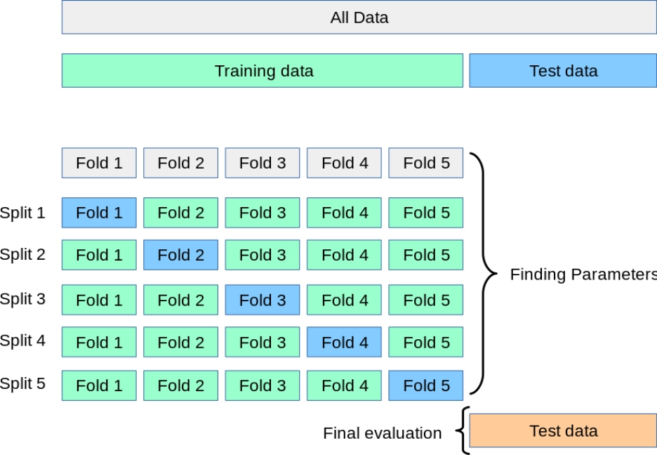
Cross-validation serves as a basic technique which machine learning models use to evaluate their performance. The procedure requires dividing data into various training sets and testing sets to determine how well the model performs with new data. The k-fold cross-validation method requires data to be divided into k equal sections which are known as folds. The test set uses one fold while the remaining folds create the training set. The test set uses one fold while the remaining folds create the training set. 

Traditional cross-validation requires data points to follow independent and identical distribution patterns which include randomization. The standard methods cannot be applied to sequential time series data because time order needs to be maintained. 

Read more: Cross Validation Techniques

Understanding Time Series Cross-Validation

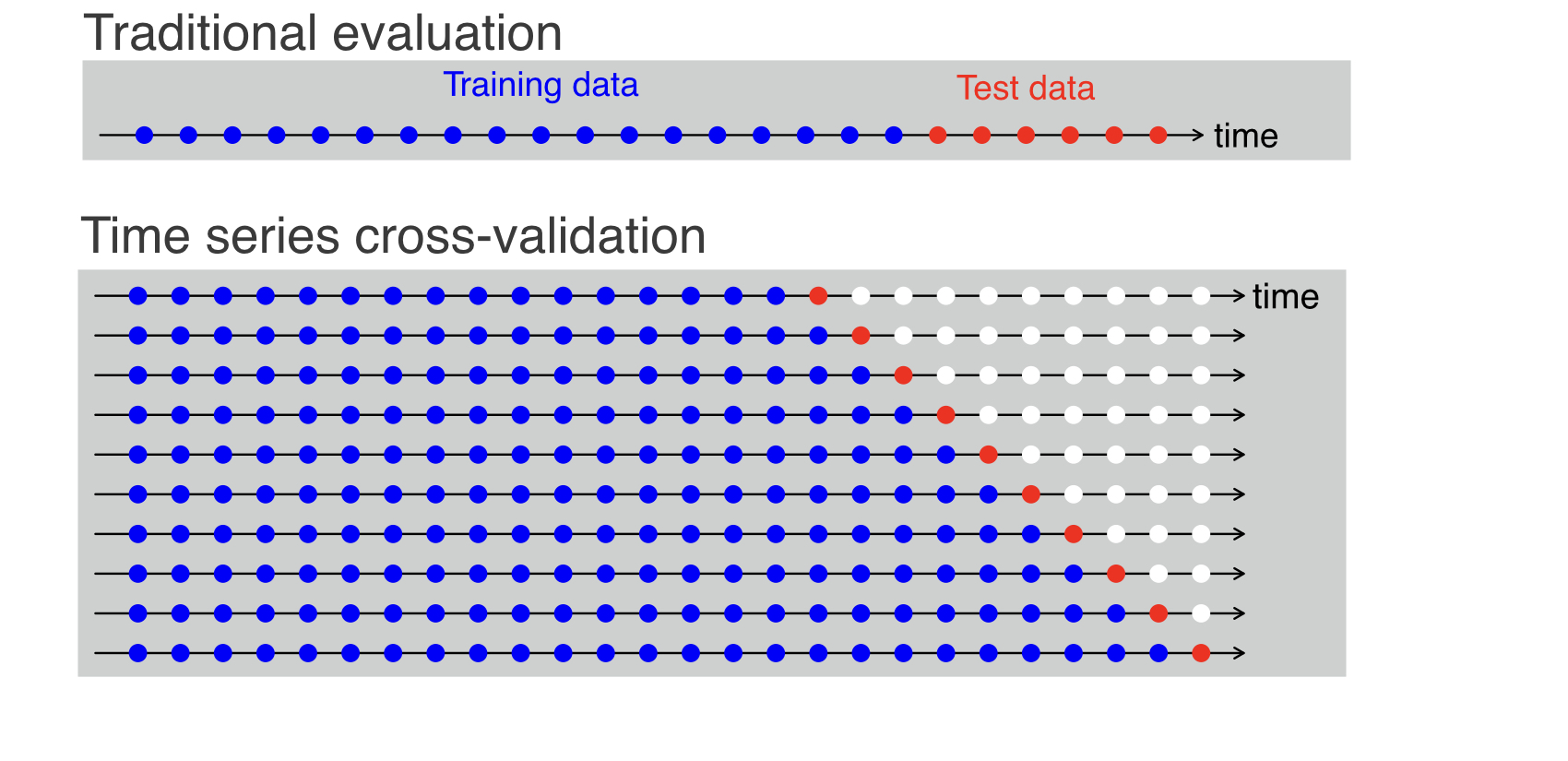
Time series cross-validation adapts standard CV to sequential data by enforcing the chronological order of observations. The method generates multiple train-test splits through its process which tests each set after their corresponding training periods. The earliest time points cannot serve as a test set because the model has no prior data to train on. The evaluation of forecasting accuracy uses time-based folds to average metrics which include MSE through their measurement. 

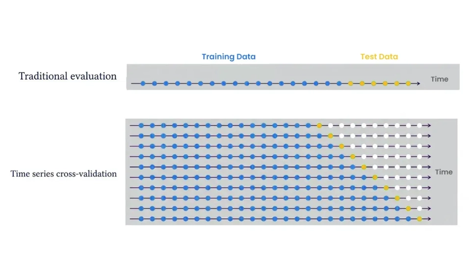
The figure above shows a basic rolling-origin cross-validation system which tests model performance by training on blue data until time t and testing on the subsequent orange data point. The training window then “rolls forward” and repeats. The walk-forward approach simulates actual forecasting by training the model on historical data and testing it on upcoming data. Through the use of multiple folds we obtain multiple error measurements which include MSE results from each fold that we can use to evaluate and compare different models. 

Model Building and Evaluation

Let’s see a practical example using Python. We use pandas to load our training data from the file train.csv while TimeSeriesSplit from scikit-learn creates sequential folds and we use statsmodels’ ARIMA to develop a forecasting model. In this example, we predict the daily mean temperature (meantemp) in our time series. The code contains comments that describe the function of each programming section. 

import pandas as pd
from sklearn.model_selection import TimeSeriesSplit
from statsmodels.tsa.arima.model import ARIMA
from sklearn.metrics import mean_squared_error
import numpy as np

# Load time series data (daily records with a datetime index)
data = pd.read_csv('train.csv', parse_dates=['date'], index_col='date')

# Focus on the target series: mean temperature
series = data['meantemp']

# Define number of splits (folds) for time series cross-validation
n_splits = 5
tscv = TimeSeriesSplit(n_splits=n_splits)

The code demonstrates how to perform cross-validation. The ARIMA model is trained on the training window for each fold and used to predict the next time period which allows calculation of MSE. The process results in five MSE values which we calculate by averaging the five MSE values obtained from each split. The forecast accuracy for the held-out data improves when the MSE value decreases. 

After completing cross-validation we can train a final model using the complete training data and test its performance on a new test dataset. The final model can be created using these steps: final_model = ARIMA(series, order=(5,1,0)).fit() and then forecast = final_model.forecast(steps=len(test)) which uses test.csv data. 

# Initialize a list to store the MSE for each fold
mse_scores = []

# Perform time series cross-validation
for train_index, test_index in tscv.split(series):
    train_data = series.iloc[train_index]
    test_data = series.iloc[test_index]

    # Fit an ARIMA(5,1,0) model to the training data
    model = ARIMA(train_data, order=(5, 1, 0))
    fitted_model = model.fit()

    # Forecast the test period (len(test_data) steps ahead)
    predictions = fitted_model.forecast(steps=len(test_data))

    # Compute and record the Mean Squared Error for this fold
    mse = mean_squared_error(test_data, predictions)
    mse_scores.append(mse)

    print(f"Mean Squared Error for current split: {mse:.3f}")

# After all folds, compute the average MSE
average_mse = np.mean(mse_scores)
print(f"Average Mean Squared Error across all splits: {average_mse:.3f}")

Importance in Forecasting & Machine Learning

The proper implementation of cross-validation methods stands as an essential requirement for accurate time series forecasts. The method tests model capabilities to predict upcoming information which the model has not yet encountered. The process of model selection through cross-validation enables us to identify the model which demonstrates better capabilities for generalizing its performance. Time series CV delivers multiple error assessments which demonstrate distinct patterns of performance compared to a single train-test split. 

The process of walk-forward validation requires the model to undergo retraining during each fold which serves as a rehearsal for actual system operation. The system tests model strength through minor changes in input data while consistent results across multiple folds show system stability. Time series cross-validation provides more accurate evaluation results while assisting in optimal model and hyperparameter identification compared to a standard data split method. 

Challenges With Cross-Validation in Time Series

Time series cross-validation introduces its own challenges. It acts as an effective detection tool. Non-stationarity (concept drift) represents another challenge because model performance will change across different folds when the underlying pattern experiences regime shifts. The cross-validation process shows this pattern through its demonstration of rising errors during the later folds. 

Other challenges include: 

• Limited data in early folds: The first folds have very little training data, which can make initial forecasts unreliable. 
• Overlap between folds: The training sets in each successive fold increase in size, which creates dependence. The error estimates between folds show correlation, which results in an underestimation of actual uncertainty. 
• Computational cost: Time series CV requires the model to undergo retraining for each fold, which becomes costly when dealing with intricate models or extensive data sets. 
• Seasonality and window choice: Your data requires specific window sizes and split points because it exhibits both strong seasonal patterns and structural changes. 

Conclusion

Time series cross-validation provides accurate assessment results which reflect actual model performance. The method maintains chronological sequence of events while stopping data extraction and simulating actual system usage situations. The testing procedure causes advanced models to break down because they cannot handle new test material. 

You can create strong forecasting systems through walk-forward validation and appropriate metric selection while preventing feature leakage. Time series machine learning requires proper validation regardless of whether you use ARIMA or LSTM or gradient boosting models. 

Frequently Asked Questions

Vipin Vashisth

Hello! I'm Vipin, a passionate data science and machine learning enthusiast with a strong foundation in data analysis, machine learning algorithms, and programming. I have hands-on experience in building models, managing messy data, and solving real-world problems. My goal is to apply data-driven insights to create practical solutions that drive results. I'm eager to contribute my skills in a collaborative environment while continuing to learn and grow in the fields of Data Science, Machine Learning, and NLP.