You probably use Google on a daily basis, and nowadays, you might have noticed AI-powered search results that compile answers from multiple sources. But you might have wondered how the AI can gather all this information and respond at such blazing speeds, especially when compared to the medium-sized and large models we typically use. Smaller models are, of course, faster in response, but they are not trained on as large a corpus as bigger parameter models.
Hence, several approaches have been proposed to speed up responses, such as Mixture of Experts, which activates only a subset of the model’s weights, making inference faster. In this blog, however, we will focus on a particularly effective strategy that significantly speeds up LLM inference without compromising output quality. This technique is known as Speculative Decoding.
Table of contents
What normally happens?
In a typical LLM generation process, we go through two main steps:
- Forward Pass
- Decoding Phase
The two steps work as follows:
- During the forward pass, the input text is tokenised and fed into the LLM. As it passes through each layer of the model, the input gets transformed, and in the end, the model outputs a probability distribution over possible next tokens (i.e., each token with its corresponding probability).
- During the decoding phase, we select the next token from this distribution. This can be done either by choosing the highest probability token (greedy decoding) or by sampling from the top probable tokens (top-p or nucleus sampling kinda).
Once a token is selected, we append it to the input sequence(prefix string) and run another forward pass through the model to generate the next token. So, if we are using a large model with, say, 70 billion parameters, we need to perform a full forward pass through the entire model for every single token generated. This repeated computation makes the process time-consuming.
In simple terms, autoregressive models work like dominoes; token 100 cannot be generated until all the preceding tokens are generated. Each token requires a full forward pass through the network. So, generating 100 tokens at 20 ms per token results in about a 2-second delay, and each token must wait for all previous tokens to be processed. That’s quite expensive in terms of latency.
How Speculative Decoding helps?
Here, we use two models: a large LLM (the target model) and a smaller model (often a distilled version), which we call the draft model. The key idea is that the smaller model quickly proposes tokens that are easier and more predictable (like common words), while the larger model ensures correctness, especially for more complex or nuanced tokens (such as domain-specific terms).
In other words, the smaller model approximates the behaviour of the larger model for most tokens, but the larger model acts as a verifier to maintain overall output quality.
The core idea of speculative decoding is:
- Draft – Generate K tokens quickly using the smaller model
- Verify – Run a single forward pass of the larger model on all K tokens in parallel
- Accept/Reject – Accept correct tokens and replace incorrect ones using rejection sampling
Note: This strategy was proposed by Google Research and Google DeepMind in the paper “Accelerating LLM Decoding with Speculative Decoding.”
Diving Deeper
We know that a model typically generates one token per forward pass. However, we can also feed multiple tokens into an LLM and have them evaluated in parallel, all at once, within a single forward pass. Importantly, verifying a sequence of tokens is roughly comparable in cost to generating a single token while producing a probability distribution for each token in the sequence.
Mp = draft model (smaller model)
Mq = target model (larger model)
pf = prefix (the existing string to complete the sequence)
K = 5 (number of tokens to draft in one forward pass)
1) Draft Phase
We first run the draft model autoregressively for K (say 5) steps:
p1(x) = Mp(pf) → x1
p2(x) = Mp(pf, x1) → x2
…
p5(x) = Mp(pf, x1, x2, x3, x4) → x5
At each step, the model takes the prefix along with previously generated tokens and outputs a probability distribution over the vocabulary (corpus). We then sample from this distribution to obtain the next token, just like in the standard decoding process.
Let’s assume our prefix string to be:
pf = “I love SRH since …”
Here, p(x) represents the draft model’s confidence for each token from its existing vocabulary.
| Token | x₁ | x₂ | x₃ | x₄ | x₅ |
| they | have | Bhuvi | and | Virat | |
| p(x) | 0.9 | 0.8 | 0.7 | 0.9 | 0.7 |
This is the assumed probability distribution we got from our draft model. Now we move to the next step…
2) Verify Phase
Now that we have run the draft model for K steps to get a sequence of K(5) tokens. Now we will have to run our target model (large model) once in parallel. The target model will be fed the pf string and all the tokens generated by the draft model, since it will check all these tokens in parallel, and it will generate for us another set of 5 probability distributions for each of the 5 generated tokens.
q1(x), q2(x), q3(x), q4(x), q5(x), q6(x) = Mq(pf, x1, x2, x3, x4, x5)
Here, qi(x) stands as the target model’s confidence that the drafted tokens are correct.
| Token | x₁ | x₂ | x₃ | x₄ | x₅ |
| they | have | Bhuvi | and | Virat | |
| p(x) | 0.9 | 0.8 | 0.7 | 0.8 | 0.7 |
| q(x) | 0.9 | 0.8 | 0.8 | 0.8 | 0.2 |
You might notice q6(x); we’ll come back to this shortly. 🙂
Remember: – We are only generating distributions for the target model; we are not sampling from these distributions. All of the tokens we sample from are from the draft model, not the target model initially.
3) Accept / Reject (Intuition)
Next is the rejection sampling step, where we decide which tokens we try to keep and which to reject. We will loop through each token one at a time, comparing the p(x) and q(x) probabilities that the respective draft and target model have assigned.
We will be accepting or rejecting based on a simple if-else rule. For now, let’s just get a simple understanding of how rejection sampling happens, then let’s dive deeper. Realistically, this isn’t how this works out, but let’s go ahead for now… We shall cover this thing in the following section.
Case 1: if q(x) >= p(x) then accept the token
Case 2: else reject
| Token | x₁ | x₂ | x₃ | x₄ | x₅ |
| they | have | Bhuvi | and | Virat | |
| p(x) | 0.9 | 0.8 | 0.7 | 0.8 | 0.7 |
| q(x) | 0.9 | 0.8 | 0.8 | 0.8 | 0.2 |
| ✅ | ✅ | ✅ | ✅ | ❌ |
So here we see 0.9 == 0.9, so we accept the “they” token and so on until the 4th-draft token. But once we reach the 5th draft token, we see we have to reject the “Virat” token since the target model isn’t very confident in what the draft model has generated here. We accept tokens until we encounter the first rejection. Here, “Virat” is rejected since the target model assigns it a much lower probability. The target model will then replace this token with a corrected one.
So, the scenario that we have visualised is the almost best-case scenario. Let’s see the worst-case and best case scenario using the tabular form.
Worst Case Scenario
| Token | x₁ | x₂ | x₃ | x₄ | x₅ |
| ok | team | they | have | there | |
| p(x) | 0.8 | 0.9 | 0.6 | 0.7 | 0.8 |
| q(x) | 0.3 | 0.6 | 0.5 | 0.7 | 0.9 |
| ❌ | ❌ | ❌ | ❌ | ❌ |
Here, in this scenario, we witness that the first token is rejected itself, hence we will have to break away from the loop and discard all the following tokens too (no longer relevant, hence discarded). Since each token is related to its preceding token. And then the target model has to correct the x1 token, and then again the draft model will draft a new set of 5 tokens and the target model verifies it, and so the process proceeds.
So, here in the worst-case scenario, we will generate only one token at a time, which is equivalent to us running our task with the larger model, normally similar to standard decoding, without adopting speculative decoding.
Best Case Scenario
| Token | x₁ | x₂ | x₃ | x₄ | x₅ |
| they | have | Bhuvi | and | David | |
| p(x) | 0.9 | 0.8 | 0.7 | 0.8 | 0.7 |
| q(x) | 0.9 | 0.8 | 0.8 | 0.8 | 0.9 |
| ✅ | ✅ | ✅ | ✅ | ✅ |
Here, in the best case scenario, we see all the draft tokens have been accepted by the target model with flying colors and on top of this. Do you remember when we questioned why the q6(x) token was generated by the target model? So here we will get to know about this.
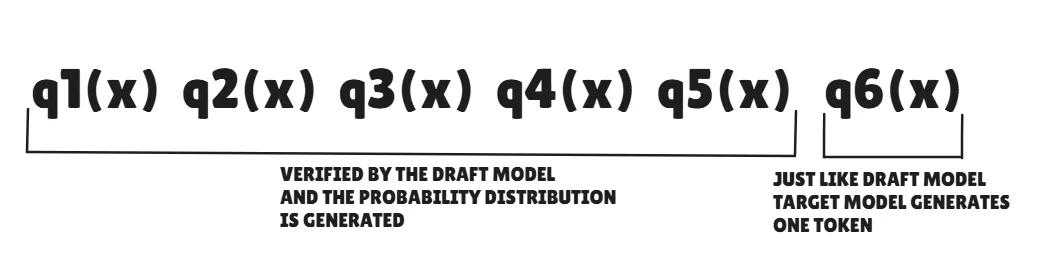
So basically, the target model takes in the prefix string, and the draft model generated tokens and verifies them. Along with the target model’s probability distribution, it gives out one token following the x5 token. So, following the tabular example we have above, we will get “Warner” as the token from the target model.
Hence, in the best-case scenario, we get K+1 tokens at one time. Whoa, that’s a huge speedup.
Speculative decoding gives ~2–3× speedup by drafting tokens and verifying them in parallel. Rejection sampling is key, ensuring output quality matches the target model despite using draft tokens.
Source: Google
How many tokens are in one pass?
Worst case: First token is rejected -> 1 token from the target model is accepted
Best case: All draft tokens are accepted -> (draft tokens) + (target model token) tokens generated [K+1]
In the DeepMind paper, it is recommended to keep K = 3 and 4. This often got them 2 to 2.5x speedup when compared to auto-regressive decoding. In the Google paper, 3 was recommended, which got them 2 to 3.4x speedup.
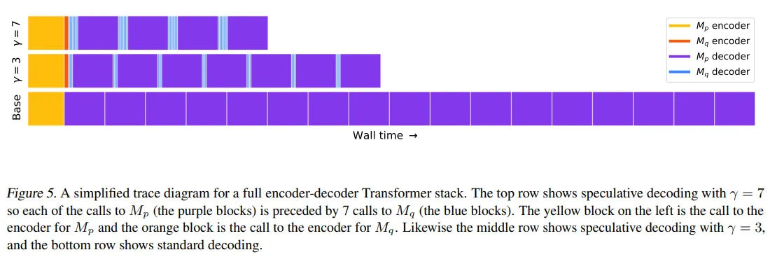
In the above image, we can see how using K = 3 or 7 has drastically reduced the latency time.
This overall helps in reducing the latency, decreases our compute costs since there is less GPU resource utilisation and boosts the memory usage, hence boosting efficiency.
Note: Verifying the draft tokens is faster than generating tokens by the target model. Also, there is a slight overhead since we are using 2 models. We will discuss different types of speculative decoding in further sections.
The Real Rejection Sampling Math
So, we went over the rejection sampling concept above, but realistically, this is how we accept or reject a certain token.
Case 1: if q(x) >= p(x), accept the token
Case 2: if q(x) < p(x) then, we accept with the probability of min(1, q(x)/p(x))
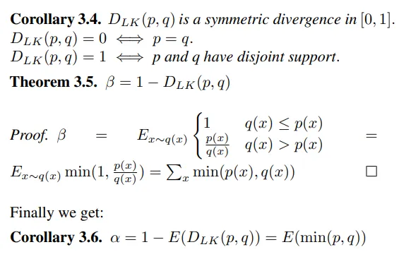
This is the algorithm used for rejection sampling in the paper.
Note: Don’t get confused between the q(x) and p(x) we used earlier and the notation used in the above image.
Visualizing Outputs
Let’s visualize this with the almost best-case scenario table we used above.
| Token | x₁ | x₂ | x₃ | x₄ | x₅ |
| they | have | Bhuvi | and | Virat | |
| p(x) | 0.9 | 0.8 | 0.7 | 0.8 | 0.7 |
| q(x) | 0.9 | 0.8 | 0.8 | 0.8 | 0.2 |
| ✅ | ✅ | ✅ | ✅ | ❌ | |
| min(1, q(x)/p(x)) | 1 | 1 | 1 | 1 | 0.29 |
Here, for the 5th token, since the value is quite low (0.29), the probability of accepting this token is very small; we are very likely to reject this draft token and sample from the target model vocabulary to replace it. So for this token, we won’t be sampling from the draft model p(x), but instead from the target model q(x), for which we already have the probability distribution.
But, we actually don’t sample from q(x) directly; instead, we sample from an adjusted distribution (q(x) − p(x)). Basically, we subtract the token probabilities across the two probability distributions and ignore the negative values, similar to a ReLU function.
Our main goal here is to sample the token from the target model distribution. So essentially, we will be sampling only from the region where the target model has higher confidence than the draft model (the reddish region).
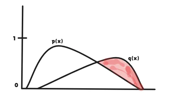
Now that you are seeing this, you might understand why we aren’t sampling directly from the q(x) probability distribution, right? But honestly, there is no information loss here. This process allows us to sample only from the portion where correction is needed. Hence, this is why speculative decoding is considered mathematically lossless.
So, now we officially understand how speculative decoding actually works. Woohoo. Now, let’s dive into the last section of this blog.
Different Approaches to Speculative Decoding
Approach 1
In this approach, we follow the same method that we implemented in the earlier examples, i.e., using two different models. These models can belong to the same organisation (like Meta, Mistral, etc.) or can also be from different organisations. The draft model generates K tokens at once, and the target model verifies all these tokens in a single forward pass. When all the draft tokens are accepted, we effectively advance K tokens for the cost of one large forward pass.
Eg, we can use 2 models from the same organisation:
- mistralai/Mistral-7B-v0.1 → mistralai/Mixtral-8x7B-v0.1
- deepseek-ai/deepseek-llm-7b-base → deepseek-ai/deepseek-llm-67b-base
- Qwen/Qwen-7B → Qwen/Qwen-72B
We can also use models from different organisations:
- meta-llama/Llama-2-7b-hf → Qwen/Qwen-72B
- meta-llama/Llama-2-13b-hf → Qwen/Qwen-72B-Chat
NOTE: Just keep in mind that cross-organisation setups usually have lower token acceptance rates due to tokeniser and distribution mismatch, so the speedups may be smaller compared to same-family pairs. It is generally preferred to use models from the same family.
Approach 2
For some use cases, hosting two separate models can be memory-intensive. In such scenarios, we can adopt the strategy of self-speculation, where the same model is used for both drafting and verification.
This does not mean we literally use two separate instances of the same model. Instead, we modify the model to behave like a smaller version during the draft phase. This can be done by reducing precision (e.g., lower-bit representations) or by selectively using only a subset of layers.
1. LayerSkip (Early Exit)
In this approach, we use only a subset of the model’s layers (e.g., Layer 1 to 12) repeatedly as a lightweight draft model for K times, and occasionally run the full model (e.g., Layer 1 to 32) once to verify all the drafted tokens. In practice, the partial model is run K times to generate K draft tokens, and then the full model is run once to verify them. This acts as a cheaper drafting mechanism while still maintaining output quality during verification. This approach typically achieves around 2x to 2.5x speedup with an acceptance rate of 75-80%.
2. EAGLE
EAGLE (Extrapolation Algorithm for Greater Language-Model Efficiency) is a learned predictor approach, where a small auxiliary model (approx 100M parameters) is trained to predict draft tokens based on the frozen model’s hidden states. This achieves around 2.5x to 3x speedup with an acceptance rate of 80-85%.
EAGLE essentially acts like a student model used for drafting. It removes the overhead of running a completely separate large draft model, while still allowing the target model to verify multiple tokens in parallel.
Another plus point of using self-speculation is that there is no latency overhead since we don’t switch models here. We can explore EAGLE and other speculative decoding techniques in more detail in a separate blog.
Conclusion
Speculative decoding works best with low batch sizes, underutilised GPUs, and long outputs (100+ tokens). It’s especially useful for predictable tasks like code generation and latency-sensitive applications where faster responses matter.
It speeds up inference by drafting tokens and verifying them in parallel, reducing latency without losing quality. Rejection sampling keeps outputs identical to the target model. New approaches like LayerSkip and EAGLE further improve efficiency, making this a practical method for scaling LLM performance.
Frequently Asked Questions
Q1. What is speculative decoding?
A. It’s a method where a smaller model drafts tokens and a larger model verifies them to speed up text generation.
Q2. How does speculative decoding reduce latency?
A. It generates multiple tokens at once and verifies them in parallel instead of processing one token per forward pass.
Q3. How does rejection sampling work in speculative decoding?
A. Tokens are accepted if q(x) ≥ p(x), otherwise accepted probabilistically using min(1, q(x)/p(x)).
Data Scientist @ Analytics Vidhya | CSE AI and ML @ VIT Chennai
Passionate about AI and machine learning, I'm eager to dive into roles as an AI/ML Engineer or Data Scientist where I can make a real impact. With a knack for quick learning and a love for teamwork, I'm excited to bring innovative solutions and cutting-edge advancements to the table. My curiosity drives me to explore AI across various fields and take the initiative to delve into data engineering, ensuring I stay ahead and deliver impactful projects.