How to use XGBoost algorithm in R in easy steps

Introduction

Are you aware that employing the XGBoost algorithm is considered a winning strategy in many data science competitions?

So, what makes it more powerful than a traditional Random Forest or Neural Network? In broad terms, it’s the efficiency, accuracy, and feasibility of this algorithm. (I’ve discussed this part in detail below in this tutorial).

In the last few years, predictive modeling has become much faster and more accurate. I remember spending long hours on feature engineering to improve the model by a few decimals. A lot of that difficult work, can now be done using better algorithms.

Technically, “XGBoost” is a short form for Extreme Gradient Boosting.  It gained popularity in data science after the famous Kaggle competition called the Otto Classification Challenge. The latest implementation on “xgboost” on R was launched in August 2015. We will refer to this version (0.4-2) in this post.

In this article, I’ve explained a simple approach to using xgboost in R. So, consider this algorithm the next time you build a model. I’m sure it would be a moment of shock and then happiness!

Overview

• Learn how to use xgboost, a powerful machine learning algorithm in R
• Check out the applications of xgboost in R by using a data set and building a machine learning model with this algorithm

What is XGBoost?

Extreme gradient boosting (xgboost) is similar to the gradient boosting framework but is more efficient. It has both linear model solver and tree learning algorithms. So, what makes it fast is that it can do parallel computation on a single machine.

This makes xgboost at least 10 times faster than existing gradient boosting implementations. It supports various objective functions, including regression, classification, and ranking.

Since it is very high in predictive power but relatively slow with implementation, “xgboost” becomes an ideal fit for many competitions. It also has additional features for doing cross-validation and finding important variables. Many parameters need to be controlled to optimize the model. We will discuss these factors in the next section.

Preparation of Data for using XGBoost

XGBoost only works with numeric vectors. Yes! you need to work on data types here.

Therefore, you need to convert all other forms of data into numeric vectors. One Hot Encoding is a simple method to convert categorical variables into numeric vectors. This term emanates from digital circuit language, which means an array of binary signals, and the only legal values are 0s and 1s.

In R, one hot encoding is quite easy. This step (shown below) will essentially make a sparse matrix using flags on every possible value of that variable. A sparse Matrix is a matrix where most of the values are zeros. Conversely, a dense matrix is a matrix where most values are non-zero.

Let’s assume you have a dataset named ‘campaign’ and want to convert all categorical variables except the response variable into such flags. Here is how you do it :

sparse_matrix <- sparse.model.matrix(response ~ .-1, data = campaign)

Now, let’s break down this code as follows:

• “sparse.model.matrix” is the command, and all other inputs inside parentheses are parameters.
• The parameter “response” says this statement should ignore the “response” variable.
• “-1” removes an extra column, which this command creates as the first column.
• And finally, you specify the dataset name.

To convert the target variables as well, you can use the following code:

output_vector = df[,response] == "Responder"

Here is what the code does:

• set output_vector to 0
• set output_vector to 1 for rows where the response is "Responder" is TRUE ;
• return  output_vector.

Building Model using Xgboost on R

Here are simple steps you can use to crack any data problem using xgboost:

Step 1: Load all the libraries

library(xgboost)
library(readr)
library(stringr)
library(caret)
library(car)

Step 2 : Load the dataset

(Here, I use bank data where we need to find whether a customer is eligible for a loan or not).

set.seed(100)
setwd("C:\\Users\\ts93856\\Desktop\\datasource")
# load data
df_train = read_csv("train_users_2.csv")
df_test = read_csv("test_users.csv")

# Loading labels of train data

labels = df_train['labels']
df_train = df_train[-grep('labels', colnames(df_train))]

# combine train and test data
df_all = rbind(df_train,df_test)

Step 3: Data Cleaning & Feature Engineering

# clean Variables :  here I clean people with age less than 14 or more than 100

df_all[df_all$age < 14 | df_all$age > 100,'age'] <- -1
df_all$age[df_all$age < 0] <- mean(df_all$age[df_all$age > 0])

# one-hot-encoding categorical features
ohe_feats = c('gender', 'education', 'employer')

dummies <- dummyVars(~ gender +  education + employer, data = df_all)
df_all_ohe <- as.data.frame(predict(dummies, newdata = df_all))
df_all_combined <- cbind(df_all[,-c(which(colnames(df_all) %in% ohe_feats))],df_all_ohe)df_all_combined$agena <- as.factor(ifelse(df_all_combined$age < 0,1,0))

I am using a list of variables in “feature_selected” to be used by the model. I have shared a quick and smart way to choose variables later in this article.

df_all_combined <- df_all_combined[,c('id',features_selected)] 
# split train and test
X = df_all_combined[df_all_combined$id %in% df_train$id,]
y <- recode(labels$labels,"'True'=1; 'False'=0)
X_test = df_all_combined[df_all_combined$id %in% df_test$id,]

Step 4: Tune and Run the model

xgb <- xgboost(data = data.matrix(X[,-1]), 
 label = y, 
 eta = 0.1,
 max_depth = 15, 
 nround=25, 
 subsample = 0.5,
 colsample_bytree = 0.5,
 seed = 1,
 eval_metric = "merror",
 objective = "multi:softprob",
 num_class = 12,
 nthread = 3
)

Step 5: Score the Test Population

And that’s it! You now have an object “xgb” which is an xgboost model. Here is how you score a test population :

# predict values in test set
y_pred <- predict(xgb, data.matrix(X_test[,-1]))

Parameters used in Xgboost

I understand, by now, you would be highly curious to know about various parameters used in xgboost model. So, there are three types of parameters: General Parameters, Booster Parameters, and Task Parameters.

• General parameters refer to which booster we are using to do boosting. The commonly used are tree or linear model
• Booster parameters depend on which booster you have chosen
• Learning Task parameters that decide on the learning scenario, for example, regression tasks may use different parameters with ranking tasks.

Let’s understand these parameters in detail. I require you to pay attention here. This is the most critical aspect of implementing the xgboost algorithm:

General Parameters

• silent : The default value is 0. You need to specify 0 for printing running messages, 1 for silent mode.
• booster : The default value is gbtree. You need to specify the booster to use: gbtree (tree based) or gblinear (linear function).
• num_pbuffer : This is set automatically by xgboost, no need to be set by user. Read documentation of xgboost for more details.
• num_feature : This is set automatically by xgboost, no need to be set by user.

Booster Parameters

The tree specific parameters –

• eta : The default value is set to 0.3. You need to specify step size shrinkage used in update to prevents overfitting. After each boosting step, we can directly get the weights of new features. and eta actually shrinks the feature weights to make the boosting process more conservative. The range is 0 to 1. Low eta value means model is more robust to overfitting.
• gamma : The default value is set to 0. You need to specify minimum loss reduction required to make a further partition on a leaf node of the tree. The larger, the more conservative the algorithm will be. The range is 0 to ∞. Larger the gamma more conservative the algorithm is.
• max_depth : The default value is set to 6. You need to specify the maximum depth of a tree. The range is 1 to ∞.
• min_child_weight : The default value is set to 1. You need to specify the minimum sum of instance weight(hessian) needed in a child. If the tree partition step results in a leaf node with the sum of instance weight less than min_child_weight, then the building process will give up further partitioning. In linear regression mode, this simply corresponds to minimum number of instances needed to be in each node. The larger, the more conservative the algorithm will be. The range is 0 to ∞.
• max_delta_step : The default value is set to 0. Maximum delta step we allow each tree’s weight estimation to be. If the value is set to 0, it means there is no constraint. If it is set to a positive value, it can help making the update step more conservative. Usually this parameter is not needed, but it might help in logistic regression when class is extremely imbalanced. Set it to value of 1-10 might help control the update.The range is 0 to ∞.
• subsample : The default value is set to 1. You need to specify the subsample ratio of the training instance. Setting it to 0.5 means that XGBoost randomly collected half of the data instances to grow trees and this will prevent overfitting. The range is 0 to 1.
• colsample_bytree : The default value is set to 1. You need to specify the subsample ratio of columns when constructing each tree. The range is 0 to 1.

Linear Booster Specific Parameters

• lambda and alpha : These are regularization terms on weights. Lambda default value assumed is 1, and alpha is 0.
• lambda_bias : L2 regularization term on bias and has a default value of 0.

Learning Task Parameters

• base_score : The default value is set to 0.5 . You need to specify the initial prediction score of all instances, global bias.
• objective : The default value is set to reg:linear . You need to specify the type of learner you want which includes linear regression, logistic regression, poisson regression etc.
• eval_metric : You need to specify the evaluation metrics for validation data, a default metric will be assigned according to objective( rmse for regression, and error for classification, mean average precision for ranking
• seed : As always here you specify the seed to reproduce the same set of outputs.

Advanced functionality of xgboost

Compared to other machine learning techniques, I find implementing xgboost really simple. You already have a model if you have done all we have until now.

Let’s take it one step further and try to find the importance of the variable in the model and subset our variable list.

# Lets start with finding what the actual tree looks like

model <- xgb.dump(xgb, with.stats = T)
model[1:10] #This statement prints top 10 nodes of the model

# Get the feature real names
names <- dimnames(data.matrix(X[,-1]))[[2]]

# Compute feature importance matrix
importance_matrix <- xgb.importance(names, model = xgb)
# Nice graph
xgb.plot.importance(importance_matrix[1:10,])

#In case last step does not work for you because of a version issue, you can try following :
barplot(importance_matrix[,1])

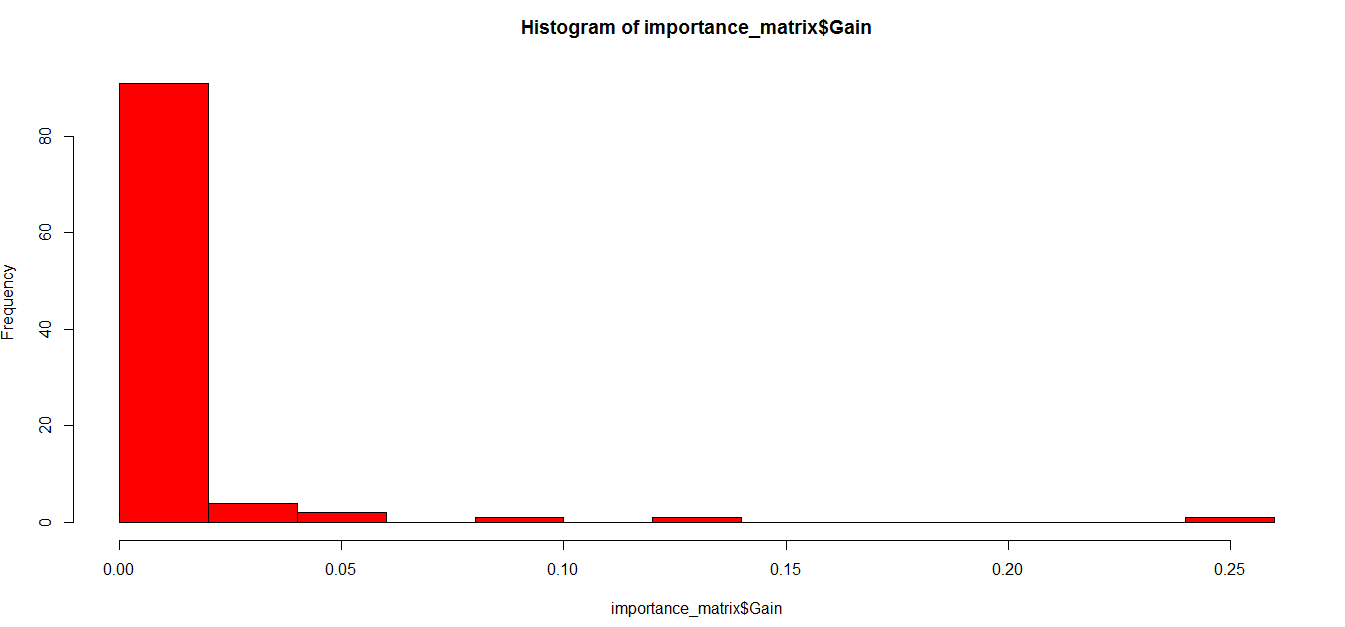
As you can observe, many variables are just not worth using into our model. You can conveniently remove these variables and run the model again. This time you can expect a better accuracy.

Testing whether the results make sense

Let’s assume, Age was the variable which came out to be most important from the above analysis. Here is a simple chi-square test which you can do to see whether the variable is actually important or not.

test <- chisq.test(train$Age, output_vector)
print(test)

We can do the same process for all important variables. This will bring out the fact whether the model has accurately identified all possible important variables or not.

End Notes

In conclusion, the XGBoost algorithm offers powerful capabilities for building numeric predictive models in both R and Python. By monitoring metrics like test error and leveraging features such as watchlist, we can iteratively refine our models for improved performance. With its versatility and efficiency, XGBoost remains a cornerstone in modern data science, enabling precise and actionable insights from complex datasets.

Frequently Asked Questions

If you like what you just read & want to continue your analytics learning, subscribe to our emails, follow us on twitter or like our facebook page.

tavish 18 Feb, 2024