Learn How to Use Support Vector Machines (SVM) for Data Science

Introduction

Mastering machine learning algorithms isn’t a myth at all. Most beginners start by learning regression. It is simple to learn and use, but does that solve our purpose? Of course not! Because there is a lot more in ML beyond logistic regression and regression problems! For instance, have you heard of support vector regression and support vector machines algorithm or SVM?

Think of machine learning algorithms as an armory packed with axes, swords, blades, bows, daggers, etc. You have various tools, but you ought to learn to use them at the right time. As an analogy, think of ‘Regression’ as a sword capable of slicing and dicing data efficiently but incapable of dealing with highly complex data. That is where ‘Support Vector Machines’ acts like a sharp knife – it works on smaller datasets, but on complex ones, it can be much stronger and more powerful in building machine learning models.

In this article, you will explore Support Vector Machines (SVM) in machine learning, including an SVM example that illustrates their functionality. We will discuss SVM code and provide a support vector machine example in Python, highlighting how these techniques can effectively classify data.

Learning Objectives

• Understand support vector machine algorithm (SVM), a popular machine learning algorithm or classification.
• Learn to implement SVM models in R and Python.
• Know the pros and cons of Support Vector Machines (SVM) and their different applications in machine learning (artificial intelligence).

What is a Support Vector Machine (SVM)?

“Support Vector Machine” (SVM) is a supervised learning machine learning algorithm that can be used for both classification or regression challenges. However, it is mostly used in classification problems, such as text classification. In the SVM algorithm, we plot each data item as a point in n-dimensional space (where n is the number of features you have), with the value of each feature being the value of a particular coordinate. Then, we perform classification by finding the optimal hyper-plane that differentiates the two classes very well (look at the below snapshot).

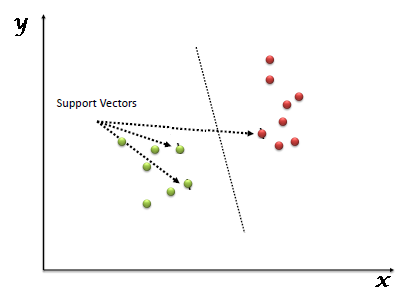
Support Vectors are simply the coordinates of individual observation, and a hyper-plane is a form of SVM visualization. The SVM classifier is a frontier that best segregates the two classes (hyper-plane/line).

How does a Support Vector Machine / SVM Work?

Above, we got accustomed to the process of segregating the two classes with a hyper-plane. Now the burning question is, “How can we identify the right hyper-plane?”. Don’t worry; it’s not as hard as you think! Let’s understand:

Identify the Right Hyper-plane

• Here, we have three hyper-planes (A, B, and C). Now, identify the right hyper-plane to classify stars and circles.
• You need to remember a thumb rule to identify the right hyper-plane: “Select the hyper-plane which segregates the two classes better.” In this scenario, hyper-plane “B” has excellently performed this job.

Another Example of Identifying the Right Hyper-plane

• Here, we have three hyper-planes (A, B, and C), and all segregate the classes well. Now, How can we identify the right hyper-plane?

• Here, maximizing the distances between the nearest data point (either class) and the hyper-plane will help us to decide the right hyper-plane. This distance is called a Margin. Let’s look at the below snapshot:

• Above, you can see that the margin for hyper-plane C is high as compared to both A and B. Hence, we name the right hyper-plane as C. Another lightning reason for selecting the hyper-plane with a higher margin is robustness. If we select a hyper-plane having a low margin, then there is a high chance of misclassification.

Another Example of Identifing the right hyper-plane

• Hint: Use the rules as discussed in the previous section to identify the right hyper-plane.

• Some of you may have selected hyper-plane B as it has a higher margin compared to A. But, here is the catch, SVM selects the hyper-plane which classifies the classes accurately prior to maximizing the margin. Here, hyper-plane B has a classification error, and A has classified all correctly. Therefore, the right hyper-plane is A.

Can we classify two classes?

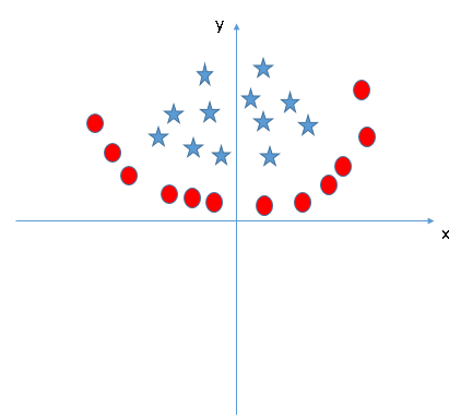
• Below, I am unable to segregate the two classes using a straight line, as one of the stars lies in the territory of the other (circle) class as an outlier.

• As I have already mentioned, one star at the other end is like an outlier for the star class. The SVM algorithm has a feature to ignore outliers and find the hyper-plane that has the maximum margin. Hence, we can say SVM classification is robust to outliers.

Find the Hyper-plane to Segregate to Classes

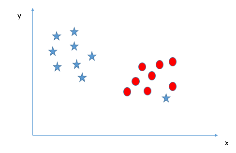
• In the scenario below, we can’t have a linear hyper-plane between the two classes, so how does SVM classify these two classes? Till now, we have only looked at the linear hyper-plane.

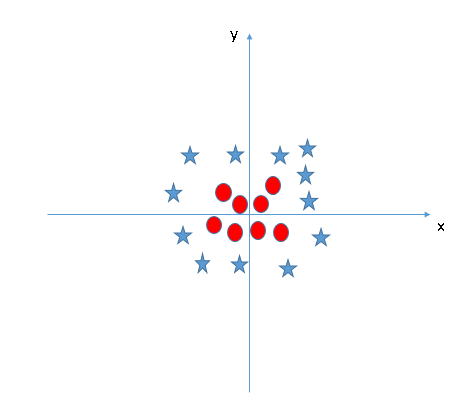
• SVM can solve this problem. Easily! Specifically, it solves this problem by introducing additional features. Here, we will add a new feature, ( z = x^2 + y^2 ). Now, let’s plot the data points on the x and z axes:

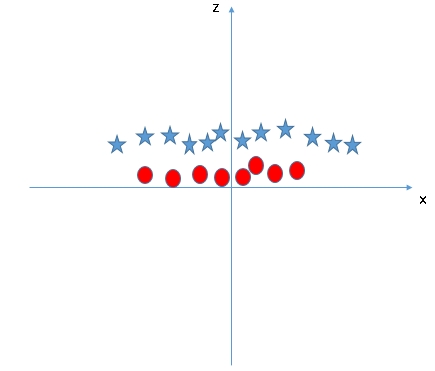
In the above plot, points to consider are:

• All values for z would always be positive because z is the squared sum of both x and y
• In the original plot, red circles appear close to the origin of the x and y axes, leading to a lower value of z. The star is relatively away from the original results due to the higher value of z.

In the SVM classifier, having a linear hyper-plane between these two classes is easy. But, another burning question that arises is if we should we need to add this feature manually to have a hyper-plane. No, the SVM  algorithm has a technique called the kernel trick. The SVM kernel transforms low-dimensional input space to a higher dimensional space, making non-separable problems separable, useful for non-linear data separation by applying complex data transformations based on labels.

When we look at the hyper-plane in the original input space, it looks like a circle:

Now, let’s look at the methods to apply the SVM classifier algorithm in a data science challenge.

You can also learn about the working of a Support Vector Machine in data mining video format from this Machine Learning certification course.

Hyperplane and Support Vectors in SVM

Hyperplane

In an SVM, a hyperplane is a decision boundary that separates different classes of data points. For instance, in a two-dimensional space, the hyperplane is a line; in a three-dimensional space, it is a plane. The goal of the SVM is to find the optimal hyperplane that maximizes the margin between the classes. The margin is defined as the distance between the hyperplane and the nearest data points from either class.

Support Vectors

Support vectors are the data points that are closest to the hyperplane. These points are critical because they determine the position and orientation of the hyperplane. If you remove a support vector, it can change the hyperplane’s position.

Types of Support Vector Machine

Linear SVM

1. Linear SVM

Linear SVM is used when the data is linearly separable, which means that the classes can be separated with a straight line (in 2D) or a flat plane (in 3D). The SVM algorithm finds the hyperplane that best divides the data into classes.

2. Non-Linear SVM

Non-Linear SVM is used when the data is not linearly separable. In such cases, SVM employs kernel functions to transform the data into a higher-dimensional space where a linear separation is possible. The algorithm then finds the optimal hyperplane in this new space.

Popular Kernel Functions in SVM

Kernels are functions that take low-dimensional input space and transform it into a higher-dimensional space. SVM can create complex decision boundaries by using kernel functions. Here are some popular kernel functions:

Linear Kernel

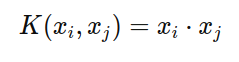
Used when the data is linearly separable.

Polynomial Kernel

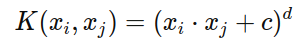
Where c is a constant, and d is the degree of the polynomial. This kernel is useful for classifying data with polynomial relationships.

Radial Basis Function (RBF) Kernel / Gaussian Kernel

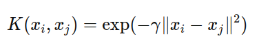
Where γ is a parameter that defines the influence of a single training example. This is one of the most popular kernels for non-linear data.

Sigmoid Kernel

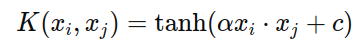
Where α and care kernel parameters. It behaves like a neural network’s activation function.

How to Implement SVM in Python and R?

In Python, scikit-learn is a widely used library for implementing machine learning algorithms. SVM algorithm is also available in the scikit-learn library, and we follow the same structure for using it(Import library, object creation, fitting model, and prediction).

Now, let us have a look at a real-life problem statement and dataset to understand how to apply SVM for classification.

Problem Statement

Dream Housing Finance company deals in all home loans. They have a presence across all urban, semi-urban, and rural areas. A customer first applies for a home loan; after that, the company validates the customer’s eligibility for a loan.

The company wants to automate the loan eligibility process (real-time) based on customer details provided while filling out an online application form. These details are Gender, Marital Status, Education, Number of Dependents, Income, Loan Amount, Credit History, and others. To automate this process, they have given a problem of identifying the customers’ segments that are eligible for loan amounts so that they can specifically target these customers. Here they have provided a partial data set.

Use the coding window below to predict the loan eligibility on the test set(new data). Try changing the hyperparameters for the linear SVM to improve the accuracy.

#Import Library
from sklearn import svm
import pandas as pd
from sklearn.metrics import accuracy_score
import warnings
warnings.filterwarnings('ignore')

#Load Train and Test datasets
#Identify feature and response variable(s) and values must be numeric and numpy arrays
train=pd.read_csv('train.csv')
train_y=train['Loan_Status']
train_x=train.drop(["Loan_Status"],axis=1)

test=pd.read_csv('test.csv')
test_y=test['Loan_Status']
test_x=test.drop(["Loan_Status"],axis=1)

# Create Linear SVM object
support = svm.LinearSVC(random_state=20)

# Train the model using the training sets and check score on test dataset
support.fit(train_x, train_y)
predicted= support.predict(test_x)
score=accuracy_score(test_y,predicted)
print("Your Model Accuracy is", score)
train.to_csv( "pred.csv")

Support Vector Machine (SVM) Code in R

The e1071 package in R is used to create Support Vector Machine in data mining with ease. It has helper functions as well as code for the Naive Bayes Classifier. The creation of a support vector machine algorithm in R and Python follows similar approaches; let’s take a look now at the following code:

#Import Library
require(e1071) #Contains the SVM 
Train <- read.csv(file.choose())
Test <- read.csv(file.choose())
# there are various options associated with SVM training; like changing kernel, gamma and C value.

# create model
model <- svm(Target~Predictor1+Predictor2+Predictor3,data=Train,kernel='linear',gamma=0.2,cost=100)

#Predict Output
preds <- predict(model,Test)
table(preds)

How to Tune the Parameters of SVM?

Tuning the parameters’ values for machine learning algorithms effectively improves model performance. Therefore, let’s look at the list of parameters available with SVM.

sklearn.svm.SVC(C=1.0, kernel='rbf', degree=3, gamma=0.0, coef0=0.0, shrinking=True, probability=False,tol=0.001, cache_size=200, class_weight=None, verbose=False, max_iter=-1, random_state=None)

I am going to discuss some important parameters having a higher impact on model performance, “kernel,” “gamma,” and “C.”

kernel: We have already discussed it. Here, we have various options available with kernel like “linear,” “rbf”, ”poly”, and others (default value is “rbf”).  Here “rbf”(radial basis function) and “poly”(polynomial kernel) are useful for non-linear hyper-plane. It’s called nonlinear svm. Let’s look at the example where we’ve used linear kernel on two features of the iris data set to classify their class.

Support Vector Machine (SVM) Code in Python

Have a Linear SVM kernel

import numpy as np
import matplotlib.pyplot as plt
from sklearn import svm, datasets

# import some data to play with
iris = datasets.load_iris()
X = iris.data[:, :2] # we only take the first two features. We could
 # avoid this ugly slicing by using a two-dim dataset
y = iris.target

# we create an instance of SVM and fit out data. We do not scale our
# data since we want to plot the support vectors
C = 1.0 # SVM regularization parameter
svc = svm.SVC(kernel='linear', C=1,gamma=0).fit(X, y)

# create a mesh to plot in
x_min, x_max = X[:, 0].min() - 1, X[:, 0].max() + 1
y_min, y_max = X[:, 1].min() - 1, X[:, 1].max() + 1
h = (x_max / x_min)/100
xx, yy = np.meshgrid(np.arange(x_min, x_max, h),
 np.arange(y_min, y_max, h))

plt.subplot(1, 1, 1)
Z = svc.predict(np.c_[xx.ravel(), yy.ravel()])
Z = Z.reshape(xx.shape)
plt.contourf(xx, yy, Z, cmap=plt.cm.Paired, alpha=0.8)

Use SVM rbf kernel

plt.scatter(X[:, 0], X[:, 1], c=y, cmap=plt.cm.Paired)
plt.xlabel('Sepal length')
plt.ylabel('Sepal width')
plt.xlim(xx.min(), xx.max())
plt.title('SVC with linear kernel')

plt.show()

Use SVM rbf kernel

Change the kernel function type to rbf in the below line and look at the impact.

svc = svm.SVC(kernel='rbf', C=1,gamma=0).fit(X, y)

I would suggest you go for a linear SVM kernel if you have a large number of features (>1000) because it is more likely that the data is linearly separable in high dimensional space. Also, you can use RBF but do not forget to cross-validate for its parameters to avoid over-fitting.

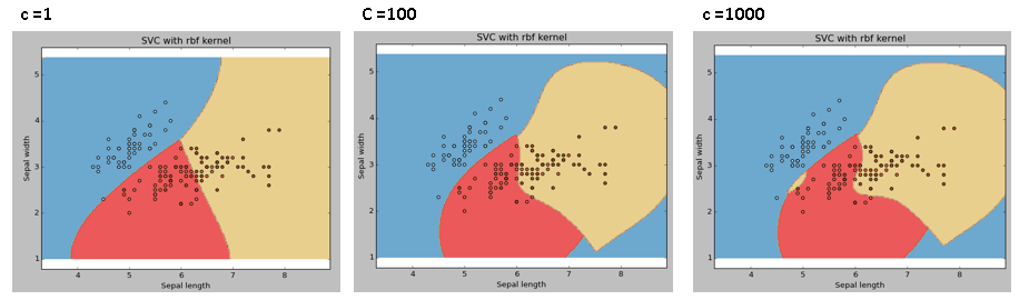
gamma: Kernel coefficient for ‘rbf’, ‘poly’, and ‘sigmoid.’ The higher value of gamma will try to fit them exactly as per the training data set, i.e., generalization error and cause over-fitting problem.

Let’s differentiate if we have gamma different gamma values like 0, 10, or 100.

svc = svm.SVC(kernel=’rbf’, C=1,gamma=0).fit(X, y)

C: Penalty parameter C of the error term. It also controls the trade-off between smooth decision boundaries and classifying the training points correctly.

We should always look at the cross-validation score to effectively combine these parameters and avoid over-fitting.

In R, SVMs algorithm can be tuned in a similar fashion as they are in Python. Mentioned below are the respective parameters for the e1071 package:

• The kernel parameter can be tuned to take “Linear”, ”Poly”, ”rbf”, etc.
• The gamma value can be tuned by setting the “Gamma” parameter.
• The C value in Python is tuned by the “Cost” parameter in R.

Pros and Cons of SVM

Pros:

• It works really well with a clear margin of separation.
• It is effective in high-dimensional spaces.
• It is effective in cases where the number of dimensions is greater than the number of samples.
• It uses a subset of the training set in the decision function (called support vectors), so it is also memory efficient.

Cons:

• It doesn’t perform well when we have a large data set because the required training time is higher.
• It also doesn’t perform very well when the data set has more noise, i.e., target classes are overlapping.
• The SVM algorithm doesn’t directly provide probability estimates; it calculates them using an expensive five-fold cross-validation. The related SVC method of the Python scikit-learn library includes this feature.

SVM Practice Problem

Find the right additional feature to have a hyper-plane for segregating the classes in the below snapshot:

Answer the variable name in the comments section below. I’ll then reveal the answer.

Conclusion

In this article, we looked at the machine learning algorithm, Support Vector Machine, in detail. We discussed the concept of its working, the process of its implementation in python and R, and the tricks to make the model more efficient by tuning its parameters. Towards the end, we also pointed out the pros and cons of the algorithm. I suggest you try solving the problem above to practice your SVM algorithm skills and also try to analyze the power of this model by tuning the parameters.

Hope you like the article on Support Vector Machines (SVM), a popular machine learning algorithm. SVM examples demonstrate its effectiveness in classifying data by finding optimal hyperplanes. Support vector machines can be implemented using SVM code in Python, making it accessible for various applications. The article covers support vector machine in machine learning with examples, showcasing its versatility in handling linear and nonlinear tasks.

Key Takeaways

• Support Vector Machine in data mining strongly and powerfully builds machine learning models with small data sets.
• You can effectively improve your model’s performance by tuning the SVM hyperparameters in Python.
• The algorithm works best when there are more dimensions than samples, and I do not recommend using it for noisy, large, or complex data sets.

Sunil Ray 12 Sep, 2024

Sunil Ray is Chief Content Officer at Analytics Vidhya, India's largest Analytics community. I am deeply passionate about understanding and explaining concepts from first principles. In my current role, I am responsible for creating top notch content for Analytics Vidhya including its courses, conferences, blogs and Competitions. I thrive in fast paced environment and love building and scaling products which unleash huge value for customers using data and technology. Over the last 6 years, I have built the content team and created multiple data products at Analytics Vidhya. Prior to Analytics Vidhya, I have 7+ years of experience working with several insurance companies like Max Life, Max Bupa, Birla Sun Life & Aviva Life Insurance in different data roles. Industry exposure: Insurance, and EdTech Major capabilities: Content Development, Product Management, Analytics, Growth Strategy.