Support Vector Machine: Introduction

This article was published as a part of the Data Science Blogathon

Introduction

In this article, we will be discussing Support Vector Machines. Before we proceed, I hope you already have some prior knowledge about Linear Regression and Logistic Regression. If you want to learn Logistic Regression, you can click here. You can also check its implementation here. By the end of this article., you will get to know the basics involved in the Support Vector Machine.

Table of Contents:

1. What is a Support Vector Machine?

2. What is the decision rule in SVM?

3. Determining the width of the margin boundaries

4. Maximising the width

5. Determining the hyperplane in N-dimensions

What is a Support Vector Machine?

Support Vector Machine is a supervised learning algorithm that is used for both classification and regression analysis. However, data scientists prefer to use this technique primarily for classification purposes. Now, I think we should now understand what is so special about SVM. In SVM, the data points can be classified in the N-dimensional space. For example, consider the following points plotted on a 2- Dimensional plane:

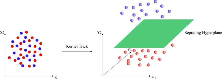
Image Source: https://www.researchgate.net/figure/SVM-classification-for-non-linearly-separable-data-points_fig4_303469788

If you look at the left part in the image, you will notice that the plotted data points are not separable with linear equations in the given plane. Does it mean that it cannot be classified? Well, “NO”! Of course, they can be classified. Just look at the image on the right side. Did you find something interesting? You guessed it right, it is separable in 3- Dimensional plane. Now the data points are separated not with the linear classifier in 2- dimensional plane, but with the hyperplane in 3- dimension.

That is why SVMs are so special!

What are the margin boundaries in SVM?

Now we would like our model to predict the new data very well. Of course, it can predict the training data, but at the very least, we would like our model to predict the validation set data very accurately.

Now, imagine the points plotted in a 2-D space. Consider a decision boundary that separates the data into 2 classes very well. Now, the points which are far from the decision boundary can be easily classified into one of the groups. Now, think of those points which are very near to the decision boundary. Don’t worry! We’ll discuss it in more detail. Consider the two points A and B as shown in the figure given below:

Now we can clearly see that point B belongs to the class of green dots as it is far from the decision line. But what about A? Which class it belongs to? You might be thinking that it also belongs to the class of green dots. But that’s not true. What if the decision boundary changes? See the figure given below:

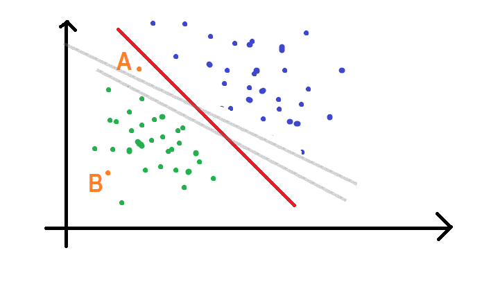
Now if we consider the grey line as our decision boundary, point A is classified as a blue point. On the other hand, it is classified as a green point if we consider the thick red line to be our decision boundary. Now we are in trouble! To avoid this ambiguity, I would like to bring the concept of “margin boundaries”.

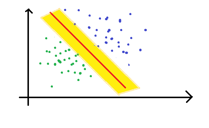
A margin boundary is a hyperplane that maximizes the margin between two classes. The decision boundary lies at the middle of the two margin boundaries. The two margin boundaries move till they encounter the first point of a class. To avoid error, we always maximize the width of the margin boundary. It will be discussed in further sections.

What is the decision rule in SVM?

Let us consider the vector w to be perpendicular to the decision boundary (note that margin boundaries and decision boundaries are parallel lines.) We have an unknown vector (point) u and we have to check whether it lies on the green side or the blue side of the line. This can be done using a decision rule that can help us to find its correct class. It is as follows:

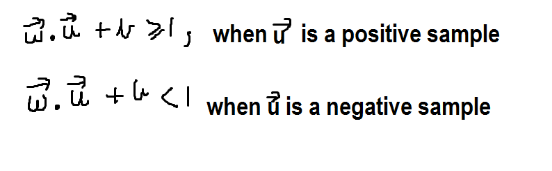
Please note that ‘b’ in the above two equations is constant.

But we see that these two equations won’t be helpful till we have a single equation. To convert the above two equations into a single equation, we again define a variable y which can take a value of either 1 or -1. This variable y is multiplied to both the equations given above, here’s the result:

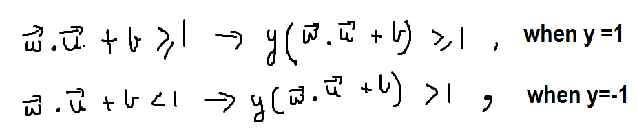
Now you see that the two equations turned out be the same when multiplied by y.

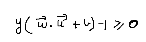
Now our final decision rule turns out to be as follows:

Determine the width of margin boundaries

As we already discussed at the beginning of the article that we want to maximize our width to avoid an error. So the time has come to find out the way for calculating the width of margin boundaries.

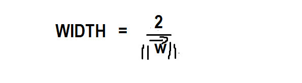
From the above equation, it is clear that the width is equal to the reciprocal of the magnitude of the vector w. Since 2 is a constant in the numerator, we can ignore it and keep the numerator equal to 1

Maximizing the Width

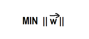
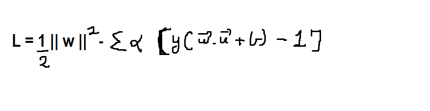
Now, we have already found the width in the above section. As I have already mentioned the width has to be maximized till we encounter any point of each of the classes. Now, to maximize the width, we actually have to minimize the following equation:

Now we will minimize it using the Lagrangian method which is as follows:

Once we differentiate it w.r.t. b and w, we get,

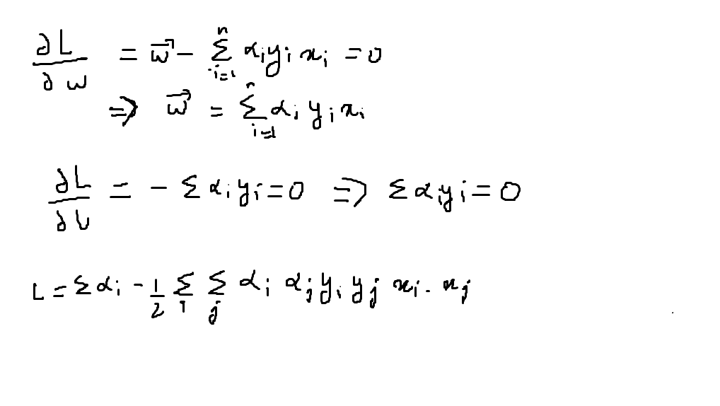
Now we have reached the end of this article but not completely. What we see in the above picture is that L has turned out to be a dot product of x_i and x_j.

NOw let’s implement SVM.

Implementation of SVM using sci-kit learn

Now its time for us to look for the implementation of support vector machines using the sklearn library:

First, we’ll introduce the dataset in our IDE:

Python Code:

import matplotlib.pyplot as plt
from sklearn import svm
import pandas as pd
import numpy as np
from sklearn.model_selection import train_test_split, GridSearchCV
loan= pd.read_csv("loan_dataset.csv")
print(loan.head())

Now you will notice that there are a lot of categorical columns which has to be converted to binary column:

loan["total_income"]=loan["ApplicantIncome"]+loan["CoapplicantIncome"]

 #converting different categorical/object values to float/int here it is float value
 loan['Gender_bool']=loan['Gender'].map({'Female':0,'Male':1})
 loan['Married_bool']=loan['Married'].map({'No':0,'Yes':1})
 loan['Education_bool']=loan['Education'].map({'Not Graduate':0,'Graduate':1})
 loan['Self_Employed_bool']=loan['Self_Employed'].map({'No':0,'Yes':1})
 loan['Property_Area_bool']=loan['Property_Area'].map({'Rural':0,'Urban':2, 'Semiurban':1})
 loan['Status_New']=loan['Loan_Status'].map({'N':0,'Y':1})

Now our task is to fill the missing values in the columns such that all categorical values are filled with mode and continuous values with the median:

#filling missing values with mode for caTEGORICAL TYPE of columns
 loan['Married_bool']=loan['Married_bool'].fillna(loan['Married_bool'].mode()[0])
 loan['Self_Employed_bool']=loan['Self_Employed_bool'].fillna(loan['Self_Employed_bool'].mode()[0])
 loan['Gender_bool']=loan['Gender_bool'].fillna(loan['Gender_bool'].mode()[0])
 loan['Dependents']=loan['Dependents'].fillna(loan['Dependents'].mode()[0])
 loan["Dependents"].replace("3+", 3,inplace=True)
 loan["CoapplicantIncome"]=loan["CoapplicantIncome"].fillna(loan["CoapplicantIncome"].median())
 loan["LoanAmount"]=loan["LoanAmount"].fillna(loan["LoanAmount"].median())
 loan["Loan_Amount_Term"]=loan["Loan_Amount_Term"].fillna(loan["Loan_Amount_Term"].median())
 loan["Credit_History"]=loan["Credit_History"].fillna(loan["Credit_History"].mode()[0])

Now we will drop the categorical columns which are not in binary form:

loan.drop("Gender", inplace=True, axis=1)
 loan.drop("Married", inplace=True, axis=1)
 loan.drop("Education", inplace=True, axis=1)
 loan.drop("Self_Employed", inplace=True, axis=1)
 loan.drop("Property_Area", inplace=True, axis=1)
 loan.drop("Loan_Status", inplace=True, axis=1)
 loan.drop("ApplicantIncome", inplace=True, axis=1)
 loan.drop("CoapplicantIncome", inplace=True, axis=1)

Now your data set looks like this:

Now our next task is to divide the data set into training set and validation set in the ratio of 80:20:

X_train, X_test, y_train, y_test = train_test_split(x_feat,y_label, test_size = 0.2)
Now it's time to train our model with SVM:
clf = svm.SVC(kernel='linear')
clf.fit(X_train, y_train)
y_pred = clf.predict(X_test)

Here in the above code, we used a linear kernel. For the above code the accuracy, precision and recall turn out to be as follows:

from sklearn import metrics
print("Accuracy:",metrics.accuracy_score(y_test, y_pred))
print("Precision:",metrics.precision_score(y_test, y_pred))

Output is:

Accuracy: 0.7642276422764228
Precision: 0.7363636363636363
Recall: 1.0

Now we can see that we have achieved an accuracy of 76.42% which is quite good and better than what we got when we trained the same dataset with logistic regression. You can check out the implementation of logistic regression on the same dataset here.

This was the end of my article. I hope you enjoyed reading out this article. This was all about the introduction toward support vector machines.

About the Author:

Hi! I am Sarvagya Agrawal. I am pursuing B.Tech. from the Netaji Subhas University Of Technology. ML is my passion and feels proud to contribute to the community of ML learners through this platform. Feel free to contact me by visiting my website: sarvagyaagrawal.github.io

The media shown in this article are not owned by Analytics Vidhya and are used at the Author’s discretion.

Sarvagya

Hi, I'm Sarvagya Agrawal, Software Engineer, with a strong passion for utilizing technology to drive positive change in society. I believe that technology is not just a skill, but an art form that can be leveraged to transform the world.
My primary focus lies in machine learning and web development, with strong programming skills in Python. I have worked on innovative projects, including developing an AI model to calculate cardiovascular risk factors from OCTA scans using computer vision algorithms and creating an AI-based web application for calculating financial risk based on an individual's spending trends.