Enhance Model Performance through Cross Validation: A Guide in Python and R

Introduction

One of the most interesting and challenging things about data science hackathons is getting a high score on both public and private leaderboards. I have closely monitored the series of data science hackathons and found an interesting trend. cross validation using python and R trend is based on participant rankings on the public and private leaderboards.

One thing that stood out was that participants who rank higher on the public leaderboard lose their position after their ranks gets validated on the private leaderboard. Some even failed to secure rank in the top 20s on the private leaderboard (image below).

Eventually, I discovered the phenomenon which brings such ripples on the leaderboard.

Take a guess! What could be the possible reason for high variation in these ranks? In other words, why does their model lose stability when evaluated on the private leaderboard?

In this article, we will look at possible reasons for this. We will also look at the concept of cross validation using python and R and a few common methods to perform it.

Note: This article is meant for every aspiring data scientist keen to improve his/her performance in data science competitions. Each technique is followed by code snippets from both R and Python.

Why do models lose stability?

Let’s understand this using the below snapshot illustrating the fit of various models:

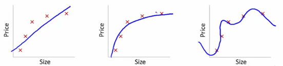
Here, we are trying to find the relationship between size and price. To achieve this, we have taken the following steps:

1. We’ve established the relationship using a linear equation for which the plots have been shown. The first plot has a high error from training data points. Therefore, this will not perform well on either public or the private leaderboard. This is an example of “Underfitting”. In this case, our model fails to capture the underlying trend of the data
2. In the second plot, we just found the right relationship between price and size, i.e., low training error and generalization of the relationship
3. In the third plot, we found a relationship which has almost zero training error. This is because the relationship is developed by considering each deviation in the data point (including noise), i.e., the model is too sensitive and captures random patterns which are present only in the current dataset. This is an example of “Overfitting”. In this relationship, there could be a high deviation between the public and private leaderboards

A common practice in data science competitions is to iterate over various models to find a better performing model. However, it becomes difficult to distinguish whether this improvement in score is coming because we are capturing the relationship better, or we are just over-fitting the data. To find the right answer for this question, we use validation techniques. This method helps us in achieving more generalized relationships.

What is Cross Validation?

Cross Validation is a technique which involves reserving a particular sample of a dataset on which you do not train the model. Later, you test your model on this sample before finalizing it.

Here are the steps involved in cross validation:

1. You reserve a sample data set
2. Train the model using the remaining part of the dataset
3. Use the reserve sample of the test (validation) set. This will help you in gauging the effectiveness of your model’s performance. If your model delivers a positive result on validation data, go ahead with the current model. It rocks!

A few common methods used for Cross Validation

There are various methods available for performing cross validation. I’ve discussed a few of them in this section.

The validation set approach

In this approach, we reserve 50% of the dataset for validation and the remaining 50% for model training. However, a major disadvantage of this approach is that since we are training a model on only 50% of the dataset, there is a huge possibility that we might miss out on some interesting information about the data which will lead to a higher bias.

Python Code:

train, validation = train_test_split(data, test_size=0.50, random_state = 5)

R Code:

set.seed(101) # Set Seed so that same sample can be reproduced in future also

# Now Selecting 50% of data as sample from total 'n' rows of the data
sample <- sample.int(n = nrow(data), size = floor(.50*nrow(data)), replace = F)
train <- data[sample, ]
test  <- data[-sample, ]

Leave one out cross validation (LOOCV)

In this approach, we reserve only one data point from the available dataset, and train the model on the rest of the data. This process iterates for each data point. This also has its own advantages and disadvantages. Let’s look at them:

• We make use of all data points, hence the bias will be low
• We repeat the cross validation process n times (where n is number of data points) which results in a higher execution time
• This approach leads to higher variation in testing model effectiveness because we test against one data point. So, our estimation gets highly influenced by the data point. If the data point turns out to be an outlier, it can lead to a higher variation

Python Code:

# importing libraries
import numpy as np
from sklearn.model_selection import LeaveOneOut

# creating the data
X = np.array([[1, 2], [3, 4]])
y = np.array([1, 2])

# Independent variable
print("\nIndependent variable :")
print(X)

# Dependent variable
print("\nDependent variable :")
print(y)

# creating the leav one out function
loo = LeaveOneOut()
loo.get_n_splits(X)

# printing the training and validation data
for train_index, test_index in loo.split(X):
    X_train, X_test = X[train_index], X[test_index]
    y_train, y_test = y[train_index], y[test_index]
    
print("\ntraining set:", X_train, y_train)
print("\nvalidation set :", X_test, y_test)


## NOTE: you can try out other validation techniques as well in this live coding window

R Code:

score = list()

LOOCV_function = function(x,label){
 for(i in 1:nrow(x)){
 training = x[-i,]
 model = #... train model on training
 validation = x[i,]
 pred = predict(model, validation[,setdiff(names(validation),label)])
 score[[i]] = rmse(pred, validation[[label]]) # score/error of ith fold
 }
 return(unlist(score)) # returns a vector
 }

LOOCV leaves one data point out. Similarly, you could leave p training examples out to have validation set of size p for each iteration. This is called LPOCV (Leave P Out Cross Validation using python and R)

k-fold cross validation

From the above two validation methods, we’ve learnt:

1. We should train the model on a large portion of the dataset. Otherwise we’ll fail to read and recognise the underlying trend in the data. This will eventually result in a higher bias
2. We also need a good ratio of testing data points. As we have seen above, less amount of data points can lead to a variance error while testing the effectiveness of the model
3. We should iterate on the training and testing process multiple times. We should change the train and test dataset distribution. This helps in validating the model effectiveness properly

Do we have a method which takes care of all these 3 requirements?

Yes! That method is known as “k-fold cross validation”. It’s easy to follow and implement. Below are the steps for it:

1. Randomly split your entire dataset into k”folds”
2. For each k-fold in your dataset, build your model on k – 1 folds of the dataset. Then, test the model to check the effectiveness for kth fold
3. Record the error you see on each of the predictions
4. Repeat this until each of the k-folds has served as the test set
5. The average of your k recorded errors is called the cross-validation error and will serve as your performance metric for the model

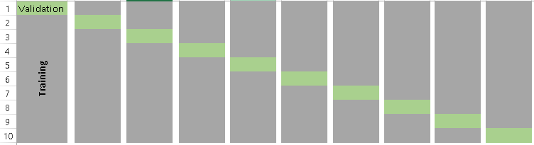
Below is the visualization of a k-fold validation when k=10.

How to choose the right value of k?

Always remember, a lower value of k is more biased, and hence undesirable. On the other hand, a higher value of K is less biased, but can suffer from large variability. It is important to know that a smaller value of k always takes us towards validation set approach, whereas a higher value of k leads to LOOCV approach.

Precisely, LOOCV is equivalent to n-fold cross validation where n is the number of training examples.

Python Code:

from sklearn.model_selection import KFold 
kf = RepeatedKFold(n_splits=5, n_repeats=10, random_state=None) 

for train_index, test_index in kf.split(X):
      print("Train:", train_index, "Validation:",test_index)
      X_train, X_test = X[train_index], X[test_index] 
      y_train, y_test = y[train_index], y[test_index]

R code:

library(caret)
data(iris)

# Define train control for k fold cross validation
train_control <- trainControl(method="cv", number=10)
# Fit Naive Bayes Model
model <- train(Species~., data=iris, trControl=train_control, method="nb")
# Summarise Results
print(model)

Stratified k-fold cross validation

Stratification is the process of rearranging the data so as to ensure that each fold is a good representative of the whole. For example, in a binary classification problem where each class comprises of 50% of the data, it is best to arrange the data such that in every fold, each class comprises of about half the instances.

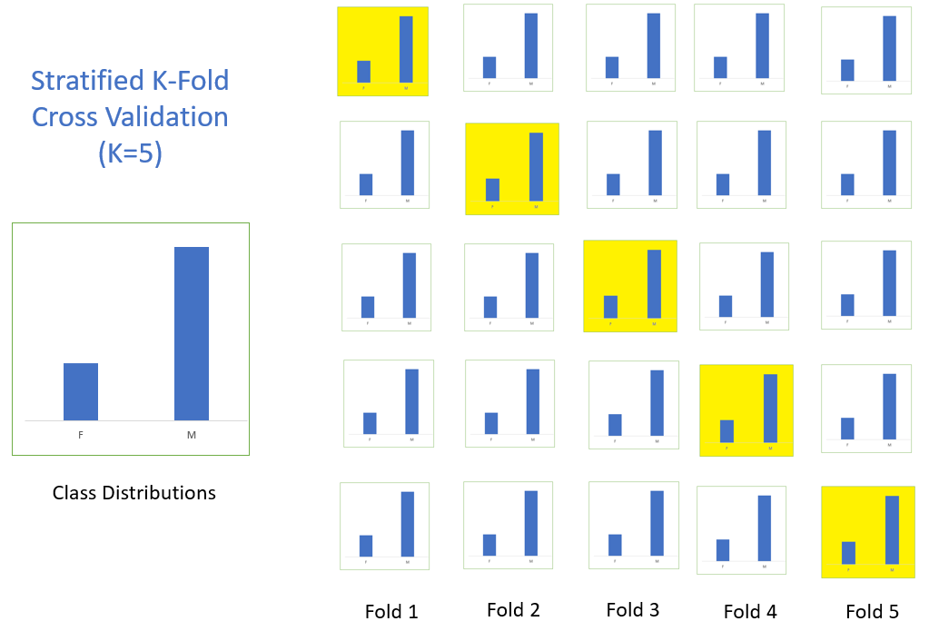
It is generally a better approach when dealing with both bias and variance. A randomly selected fold might not adequately represent the minor class, particularly in cases where there is a huge class imbalance.

Python code snippet for stratified k-fold cross validation:

from sklearn.model_selection import StratifiedKFold
skf = StratifiedKFold(n_splits=5, random_state=None)
# X is the feature set and y is the target
for train_index, test_index in skf.split(X,y): 
    print("Train:", train_index, "Validation:", val_index) 
    X_train, X_test = X[train_index], X[val_index] 
    y_train, y_test = y[train_index], y[val_index]

R Code:

library(caret)
# Folds are created on the basis of target variable
folds <- createFolds(factor(data$target), k = 10, list = FALSE)

Having said that, if the train set does not adequately represent the entire population, then using a stratified k-fold might not be the best idea. In such cases, one should use a simple k-fold cross validation with repetition.

In repeated cross-validation, the cross-validation procedure is repeated n times, yielding n random partitions of the original sample. The n results are again averaged (or otherwise combined) to produce a single estimation.

Python code for repeated k-fold cross validation:

from sklearn.model_selection import RepeatedKFold
rkf = RepeatedKFold(n_splits=5, n_repeats=10, random_state=None)
# X is the feature set and y is the target
for train_index, test_index in rkf.split(X):
     print("Train:", train_index, "Validation:", val_index)
     X_train, X_test = X[train_index], X[val_index]
     y_train, y_test = y[train_index], y[val_index]

Adversarial Validation

When dealing with real datasets, there are often cases where the test and train sets are very different. As a result, the internal cross-validation techniques might give scores that are not even in the ballpark of the test score. In such cases, adversarial validation offers an interesting solution.

The general idea is to check the degree of similarity between training and tests in terms of feature distribution. If It does not seem to be the case, we can suspect they are quite different. This intuition can be quantified by combining train and test sets, assigning 0/1 labels (0 – train, 1-test) and evaluating a binary classification task.

Let us understand, how this can be accomplished in the below steps:

Remove the target variable from the train set

train.drop(['target'], axis = 1, inplace = True)

Create a new target variable which is 1 for each row in the train set, and 0 for each row in the test set

train['is_train'] = 1
test['is_train'] = 0

Combine the train and test datasets

df = pd.concat([train, test], axis = 0)

Using the above newly created target variable, fit a classification model and predict probabilities for each row to be in the test set

y = df['is_train']; df.drop('is_train', axis = 1, inplace = True) 
# Xgboost parameters
xgb_params = {'learning_rate': 0.05, 
              'max_depth': 4,
              'subsample': 0.9,        
              'colsample_bytree': 0.9,
              'objective': 'binary:logistic',
              'silent': 1, 
              'n_estimators':100, 
              'gamma':1,         
              'min_child_weight':4}   
clf = xgb.XGBClassifier(**xgb_params, seed = 10)

Sort the train set using the calculated probabilities in step 4 and take top n% samples/rows as the validation set

probs = clf.predict_proba(x1)[:,1]
new_df = pd.DataFrame({'id':train.id, 'probs':probs})
new_df = new_df.sort_values(by = 'probs', ascending=False) # 30% validation set
val_set_ids = new_df.iloc[1:np.int(new_df.shape[0]*0.3),1]

val_set_ids will get you the ids from the train set that would constitute the validation set which is most similar to the test set. This will make your validation strategy more robust for cases where the train and test sets are highly dissimilar.

However, you must be careful while using this type of validation technique. Once the distribution of the test set changes, the validation set might no longer be a good subset to evaluate your model on.

6. Cross Validation for time series

Splitting a time-series dataset randomly does not work because the time section of your data will be messed up. For a time series forecasting problem, we perform cross validation using Python and R in the following manner.

1. Folds for time series cross valdiation are created in a forward chaining fashion
2. Suppose we have a time series for yearly consumer demand for a product during a period of n years. The folds would be created like:

fold 1: training [1], test [2]
fold 2: training [1 2], test [3]
fold 3: training [1 2 3], test [4]
fold 4: training [1 2 3 4], test [5]
fold 5: training [1 2 3 4 5], test [6]
.
.
.
fold n: training [1 2 3 ….. n-1], test [n]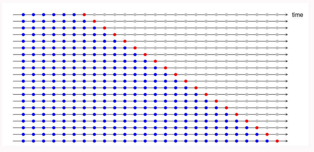

We progressively select a new train and test set. We start with a train set which has a minimum number of observations needed for fitting the model. Progressively, we change our train and test sets with each fold. In most cases, 1 step forecasts might not be very important. In such instances, the forecast origin can be shifted to allow for multi-step errors to be used. For example, in a regression problem, the following code could be used for performing cross validation using Python and R.

Python Code:

from sklearn.model_selection import TimeSeriesSplit
X = np.array([[1, 2], [3, 4], [1, 2], [3, 4]])
y = np.array([1, 2, 3, 4])
tscv = TimeSeriesSplit(n_splits=3)

for train_index, test_index in tscv.split(X):
     print("Train:", train_index, "Validation:", val_index)
     X_train, X_test = X[train_index], X[val_index]
     y_train, y_test = y[train_index], y[val_index]

TRAIN: [0] TEST: [1]
TRAIN: [0 1] TEST: [2]
TRAIN: [0 1 2] TEST: [3]

R Code:

library(fpp)
library(forecast)
e <- tsCV(ts, Arima(x, order=c(2,0,0), h=1) #CV for arima model
sqrt(mean(e^2, na.rm=TRUE)) # RMSE

h = 1 implies that we are taking the error only for 1 step ahead forecasts.

(h =4) 4-step ahead error is depicted in the below diagram. This could be used if you want to evaluate your model for multi-step forecast.

7. Custom Cross Validation Techniques

Unfortunately, there is no single method that works best for all kinds of problem statements. Often, a custom cross validation using python and R technique based on a feature, or combination of features, could be created if that gives the user stable cross validation scores while making submissions in hackathons.

For example, in the recently finished contest ‘Lord of the Machines‘ by Analytics Vidhya, the most stable validation technique used by the top finishers was using the campaign id variable.

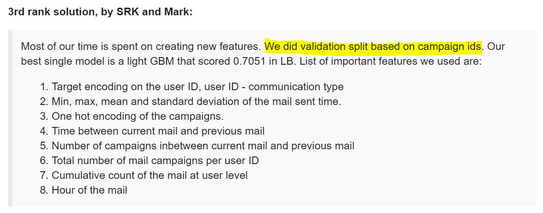
Please have a look at the problem statement and a few approaches discussed by the participants at this thread.

How to measure the model’s bias-variance?

After k-fold cross validation using python and R, we’ll get k different model estimation errors (e1, e2 …..ek). In an ideal scenario, these error values should sum up to zero. To return the model’s bias, we take the average of all the errors. Lower the average value, better the model.

Similarly for calculating the model variance, we take standard deviation of all the errors. A low value of standard deviation suggests our model does not vary a lot with different subsets of training data.

We should focus on achieving a balance between bias and variance. This can be done by reducing the variance and controlling bias to an extent. It’ll result in a better predictive model. This trade-off usually leads to building less complex predictive models as well. For understanding bias-variance trade-off in more depth, please refer to section 9 of this article.

Conclusion

In this article, we discussed about overfitting and methods like cross-validation to avoid overfitting. We also looked at different cross-validation methods like validation set approach, LOOCV, k-fold cross validation, stratified k-fold and so on, followed by each approach’s implementation in Python and R performed on the Iris dataset.

Did you find this article helpful? Please share your opinions/thoughts in the comments section below. And don’t forget to test these techniques in AV’s hackathons.

Sunil Ray 26 Feb, 2024

Sunil Ray is Chief Content Officer at Analytics Vidhya, India's largest Analytics community. I am deeply passionate about understanding and explaining concepts from first principles. In my current role, I am responsible for creating top notch content for Analytics Vidhya including its courses, conferences, blogs and Competitions. I thrive in fast paced environment and love building and scaling products which unleash huge value for customers using data and technology. Over the last 6 years, I have built the content team and created multiple data products at Analytics Vidhya. Prior to Analytics Vidhya, I have 7+ years of experience working with several insurance companies like Max Life, Max Bupa, Birla Sun Life & Aviva Life Insurance in different data roles. Industry exposure: Insurance, and EdTech Major capabilities: Content Development, Product Management, Analytics, Growth Strategy.