Future of LLMs: 3 Inventions Shaping the Next Generation of AI Models

Attention mechanism laid the foundation for transformer architectures in the field of natural language processing (NLP). Since its introduction, we have witnessed a rapid evolution in NLP. In fact, this breakthrough has marked the beginning of a new era for Generative AI and NLP as a whole. Today, companies around the world are releasing increasingly advanced LLMs. And each of these claims to set a new benchmark in performance, ultimately shaping the future of LLMs and AI in general.

To truly grasp where this future of LLMs is headed, it is important to understand some of the latest innovations influencing their development. In this article, we will explore three key advancements that are paving the path for the next generation of LLMs. These are:

• Swish Activation Function
• RoPE (Rotary Positional) Embeddings
• Infini Attention

Let’s dive into each of these topics and explore how they contribute to the evolving landscape of large language models.

Swish Activation Functions

As data scientists, we’ve encountered various activation functions. These range from the basic ones like the linear and step functions, to more advanced functions introduced with the rise of neural networks, such as tanh and the widely used ReLU. While ReLU brought significant improvements, its limitations led to the development of enhanced alternatives like Leaky ReLU, ELU, and others.

Interestingly, most of these activation functions were designed by humans. However, the Swish activation function stands out, as it was discovered by a machine. Fascinating, right? What’s more fascinating is that Swish activation plays a key role in shaping the future of LLMs. If you’re familiar with computer vision, you may have come across the YOLO-NAS model. Here is what it means.

Neural Architecture Search

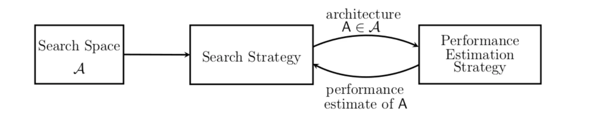
The NAS in YOLO-NAS stands for Neural Architecture Search. It is a technique developed by Google to automate the design of neural network architectures. NAS aims to identify the best-performing model configuration for a given task. This includes decisions like the number of layers and neurons.

In NAS, we define both the search space (possible architectures) and the search strategy (how we explore that space). It often focuses on metrics like accuracy or model size. Constraints are set accordingly, and numerous experiments are run to discover the optimal architecture.

Notably, EfficientNet is one of the successful architectures created using NAS, which leverages reinforcement learning to guide its search process.

This automated search for efficient neural networks was also leveraged to discover new activation functions. As a result, several promising activation function candidates were identified. Some of these include:

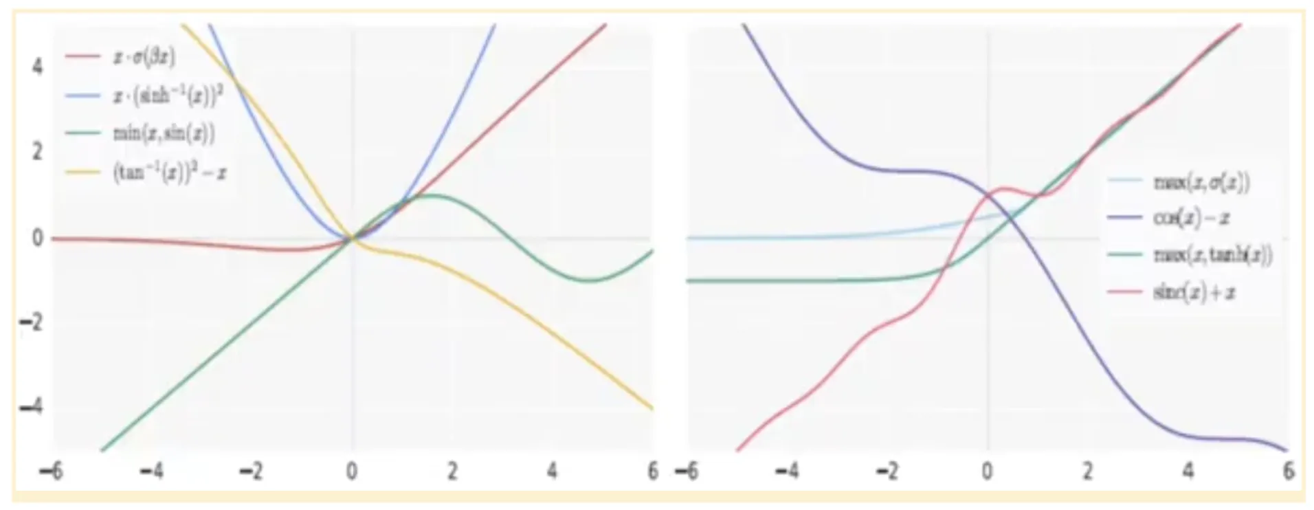
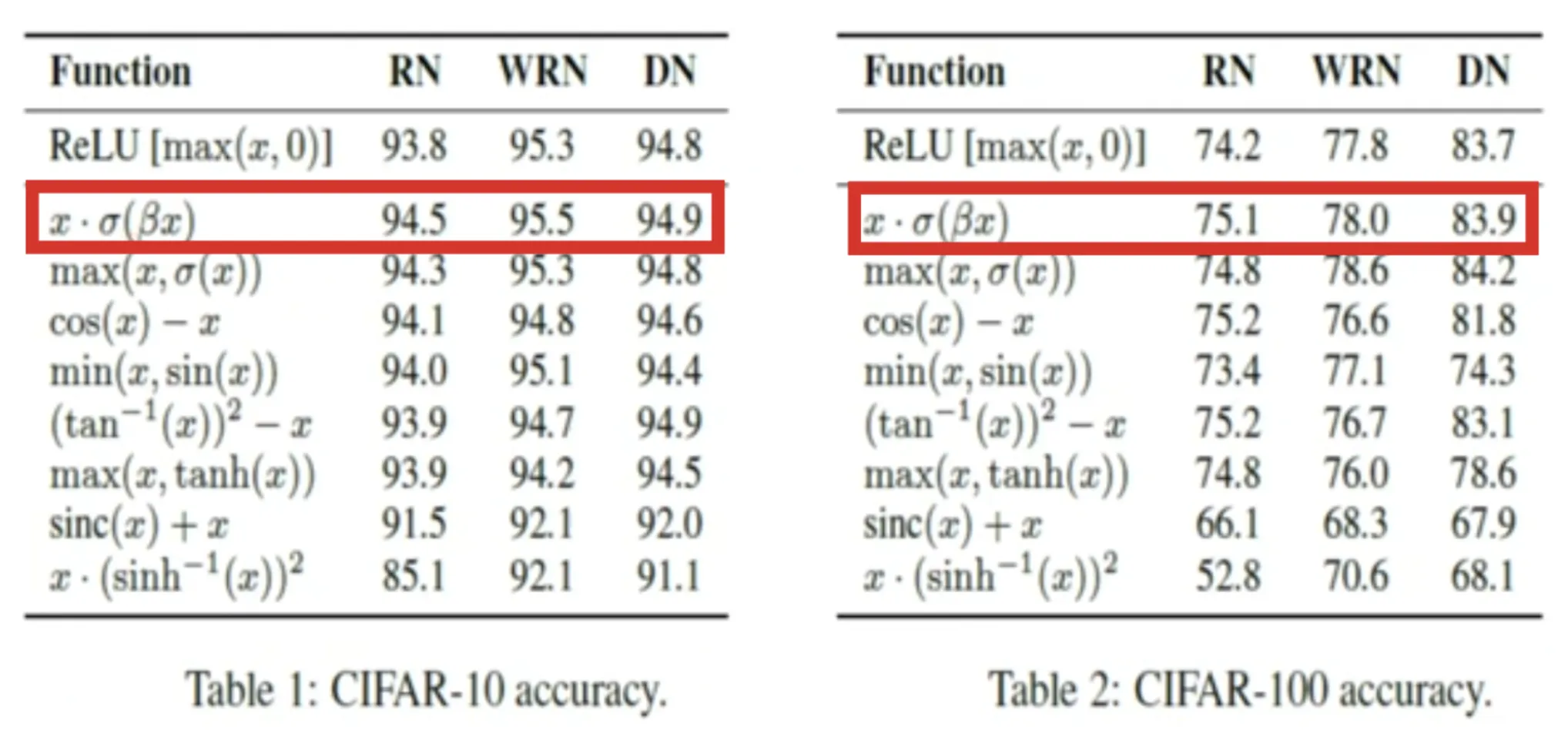
These activation functions were evaluated on benchmark datasets such as CIFAR-10 and CIFAR-100. Their performance was compared against standard models like ResNet, Wide ResNet, and DenseNet. It particularly focused on accuracy metrics compared to ReLU.

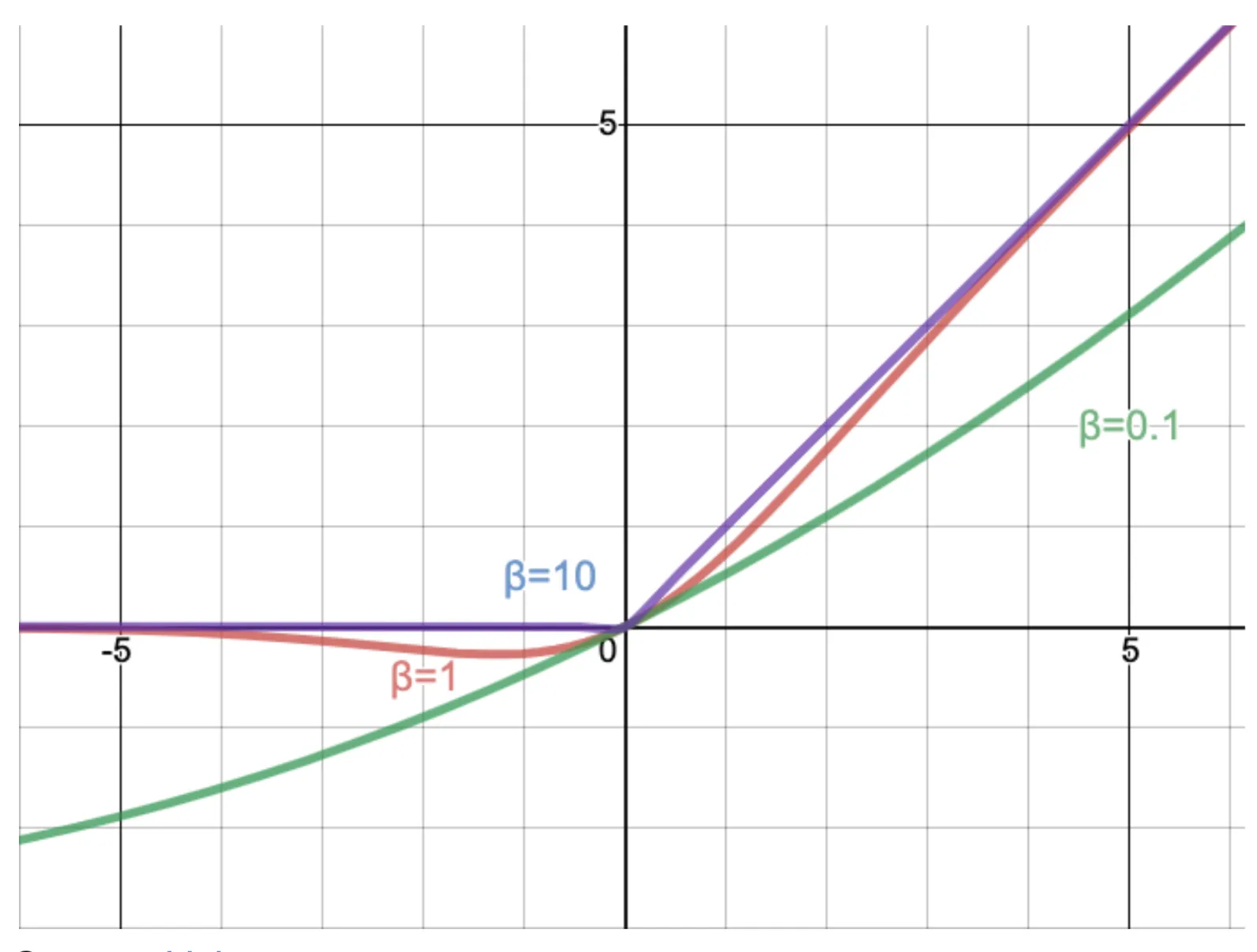
Activation functions like ReLU, Leaky ReLU, ELU, and tanh are all monotonic; they either continuously increase or decrease from the negative to the positive side of the X-axis. While Swish activation is non-monotonic. Swish activation decreases slightly initially before increasing, creating a curve that includes both downward and upward slopes.

This non-monotonicity enhances the expressive power of the network and improves gradient flow during both forward and backward passes. As a result, models using Swish activation show robustness to variations in weight initialisation and learning rates, leading to better overall training stability and performance.

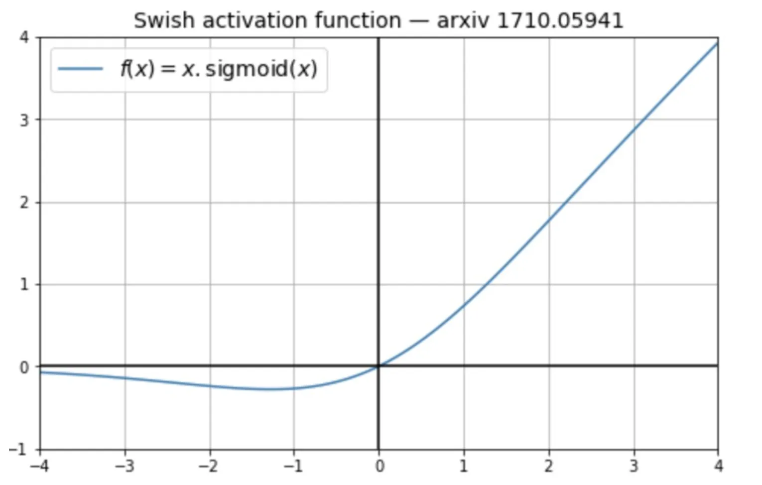
Swish activation function looks like this f(x) = x * sigmoid(βx)

Where β here is a constant or a trainable parameter.

If β < 1, it almost acts like a linear function

If β > 1, it acts more like a ReLU function

Code Implementation of the Swish Function

import numpy as np

def swish(x):
    return x * (1 / (1 + np.exp(-x)))

Where is SiLU mostly used?

SiLU is used in the Feed-Forward block of each Transformer layer, specifically after the first linear transformation, before projecting back to the model dimension.

This improves:

• Training stability
• Gradient flow
• Final model performance (especially in large-scale settings)

Swish activation Function provides a lot of desirable features, ultimately shaping the future of LLMs. These are:

• Unboundness helps get rid of the vanishing gradient problem here.
• Monotonicity is very effective as it contains both a decreasing and an increasing slope.
• It provides a smooth curve, so a gradient exists at every point.

Let’s look at how SILU is implemented within a transformer block. This code snippet provides an overview of how SiLU is utilized in forward propagation.

class TransformerBlock(nn.Module):
    def __init__(self, d_model, d_ff):
        super().__init__()
        self.attn = MultiHeadAttention(...)
        self.ffn = nn.Sequential(
            nn.Linear(d_model, d_ff),
            nn.SiLU(),                # SiLU applied here
            nn.Linear(d_ff, d_model)
        )
        self.norm1 = nn.LayerNorm(d_model)
        self.norm2 = nn.LayerNorm(d_model)

    def forward(self, x):
        x = x + self.attn(self.norm1(x))  # residual + attention
        x = x + self.ffn(self.norm2(x))   # residual + feedforward
        return x

The Feed-Forward Network (FFN) is responsible for learning complex, non-linear transformations of the token embeddings. The activation function in this FFN (historically ReLU, then GELU, and now SiLU) plays a crucial role in adding non-linearity and smooth transitions, improving learning capacity.

In Meta’s LLaMA (open-source), you’ll often find this pattern:

self.act_fn = nn.SiLU()
self.ffn = nn.Sequential(
    nn.Linear(dim, hidden_dim),
    self.act_fn,
    nn.Linear(hidden_dim, dim)
)

For instance, the Llama and Llama2 models from Meta’s Facebook Research use Swish activation/SwiGLU for their activation function. The exact details of GPT-4’s architecture are confidential. Though it is rumoured to use the sigmoid activation function (i.e., SiLU) in its loss function. Furthermore, the SiLU activation function is also used in the Ultralytics YOLO (e.g. YOLOv7) models for object detection tasks.

Now, we have understood what the Swish activation function is and where it is effectively utilised in the transformers, giving us important insights into the future of LLMs. Recently, we saw the OpenAI GPT-oss model uses a variant of the Swish activation function by the name SwiGLU. SwiGLU uses the Swish activation function, which is defined as Swish(x)=x⋅σ(x) where σ(x) is the sigmoid function, alongside a gating mechanism similar to that in GLU.

RoPE Embeddings

The Attention Is All You Need paper, published in 2017, introduced the Transformer architecture, which revolutionised the field of natural language processing. Since then, many new architectures have been proposed, though not all have proven to be equally effective. One common feature among these early transformers is their reliance on sinusoidal positional embeddings to encode the position of tokens within a sequence.

In 2022, a more effective approach to positional encoding was introduced: Rotary Positional Embeddings (RoPE). This technique has since been adopted by several large language models, including PaLM, LLaMA 1, LLaMA 2, and others. This is because of its ability to better handle longer context lengths and preserve relative position information.

You can read our in-depth article on the evolution of embeddings here.

Absolute Positional Embeddings

The previous ways of generating positional embeddings were mostly dependent on absolute positional embeddings. In absolute positional embeddings, we represent one word with its positional information. Basically we represent each word with its specific position within the sequence. And here the final tokens are made by summing the word embeddings with the positional embedding.

There were primarily 2 ways of generating positional embeddings:

1. Learned from Data: Embedding vectors are initialised randomly and then trained during the training process. This method is employed in the original transformers and in popular models like BERT, GPT, and RoBERTa.
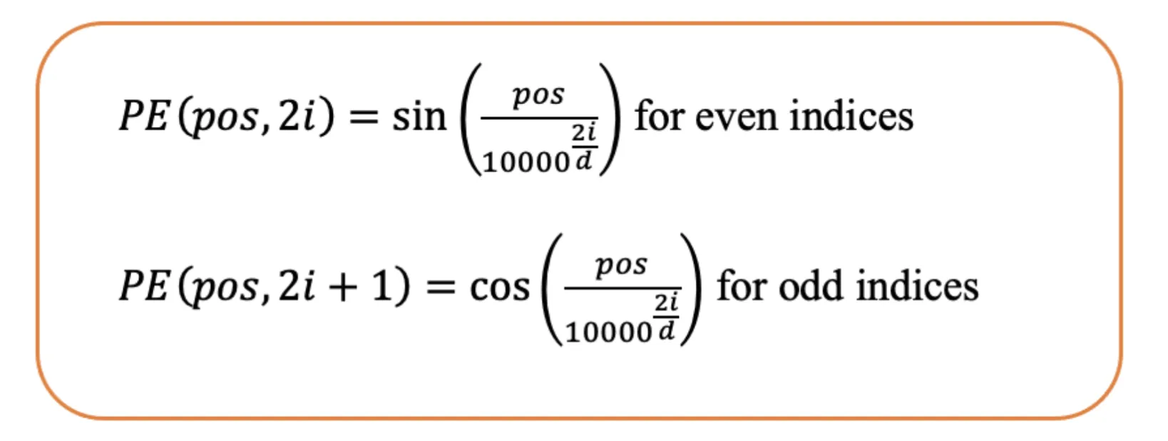
   But let’s say there is a positional vector ranging from 1 to 512. This posed a huge problem since the max length was bounded, making it hard to utilise this logic for long contexts since it couldn’t generalise it well.
2. Sinusoidal Function: It provided a unique positional embedding for each possible position within the sequence. This provides great flexibility in handling varying input sizes.
   It is also difficult to understand the pattern in the ways it shifts since both the magnitude and angle change significantly.

From different experiments, both learned and sinusoidal positional embeddings perform similarly. But one issue is that each position is treated separately. For example, the model sees the difference between position 1 and 2 as the same as between position 2 and 500, even though nearby positions are usually more related in meaning.

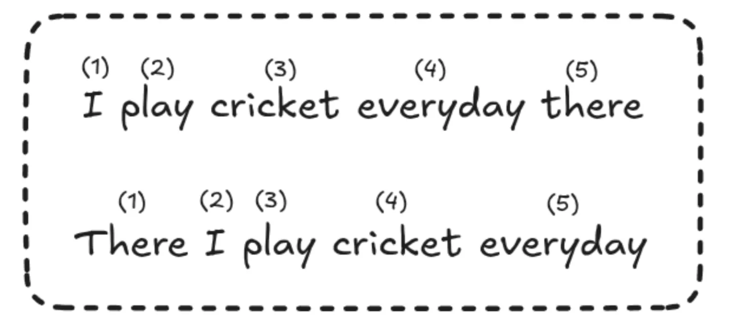
Another thing to note is that each token here gets a unique positional embedding. So, if a word is moved to a different position in the sentence, even if its meaning doesn’t change much, it still gets a completely new positional value. This can make it harder for the model to understand and generalize.

Relative Positional Embeddings

In relative positional embeddings, we don’t represent the absolute position of each token. Instead, we learn how far apart each pair of tokens is in a sentence. Since the position depends on the pair, we can’t just add the positional embedding to the token embedding like we do in absolute embeddings. Instead, we need to modify the attention mechanism itself to include this relative position information.

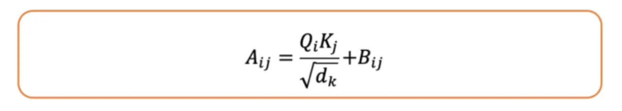
In this image, we can see the bias matrix, which denotes the relation between the words with a certain distance. Then we sum the created B matrix with the attention score matrix here.

Relative positional embeddings ensure that tokens that are, say, 3 words apart are always treated the same way, no matter where they appear in the sentence. This makes them useful for handling long sequences. However, they are slower because they need an extra step to add a bias matrix to the attention scores.

Also, since the embeddings depend on the position between each pair of tokens, we can’t easily reuse previous key-value pairs, making it hard to use key-value caching efficiently. That’s why most people do not widely use it in practice.

As we see here, relative positional embeddings help us to understand the sequence order without worrying about the exact positions and have a key role to play in the future of LLMs.

RoPE

The Rotary Positional Embeddings combine the best parts of absolute and relative positional embeddings. Here in RoPE, instead of adding a positional vector to encode the position of a word in a sequence, they propose to apply rotation to the vector.

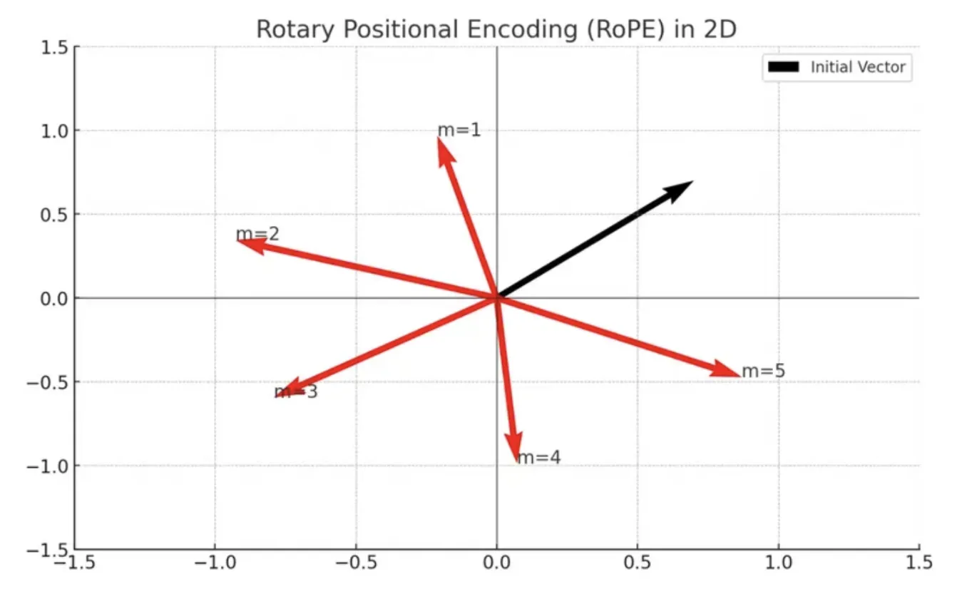
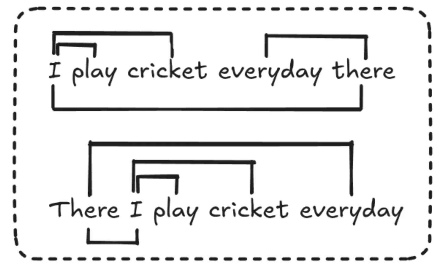
The amount we rotate is just an integer multiple of the position of the word in the sentence, so to represent the position m in the sentence. We rotate the original word vector by the angle of m times θ (theta). This has several advantages of absolute positional embeddings, like if we add more tokens to the end of a sentence stay the same, which makes them easier to catch.

The amount of rotation depends only on the token’s position in the sentence, so any number of tokens after a certain word doesn’t affect the embedding like in absolute positional embeddings.

For eg:
The cat chased the dog
Some days ago, the cat chased the dog away from here.

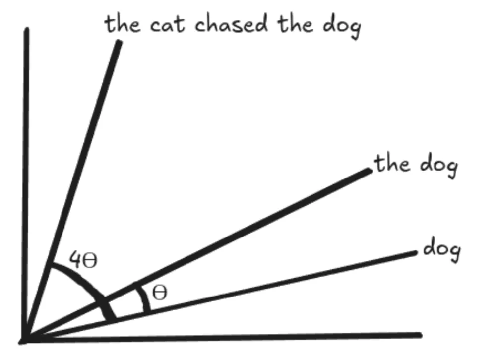
RoPE Matrix

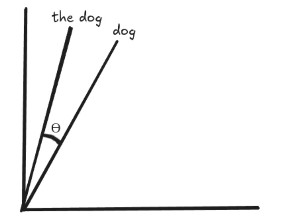
RoPE rotates the vectors for “dog” and “the dog” by the same amount, preserving the angle between them so it remains the same everywhere. This means the dot product between 2 vectors would remain the same even when we add words at the beginning or the end of those vectors, with the assumption that the distance between the vectors remains the same.

RoPE’s main idea is to rotate the query and key vectors based on their positions in the sequence.

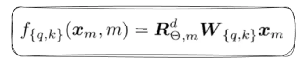
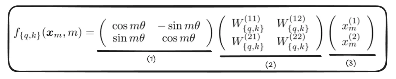
1. The Rotation Matrix, which helps rotate the vector by an angle of “m x ϴ”.
2. We first apply linear transformations to get the query and key vector, then apply a rotation matrix to preserve the rotational invariance property.
   Rotational invariance refers to the property of a system or function that remains unchanged under rotations.
   Note: We only apply rotation to query and key vectors, not the value vectors
3. This is the vector we rotate.

But in reality, the matrix is definitely not in 2D and can extend up to N dimensions like this:

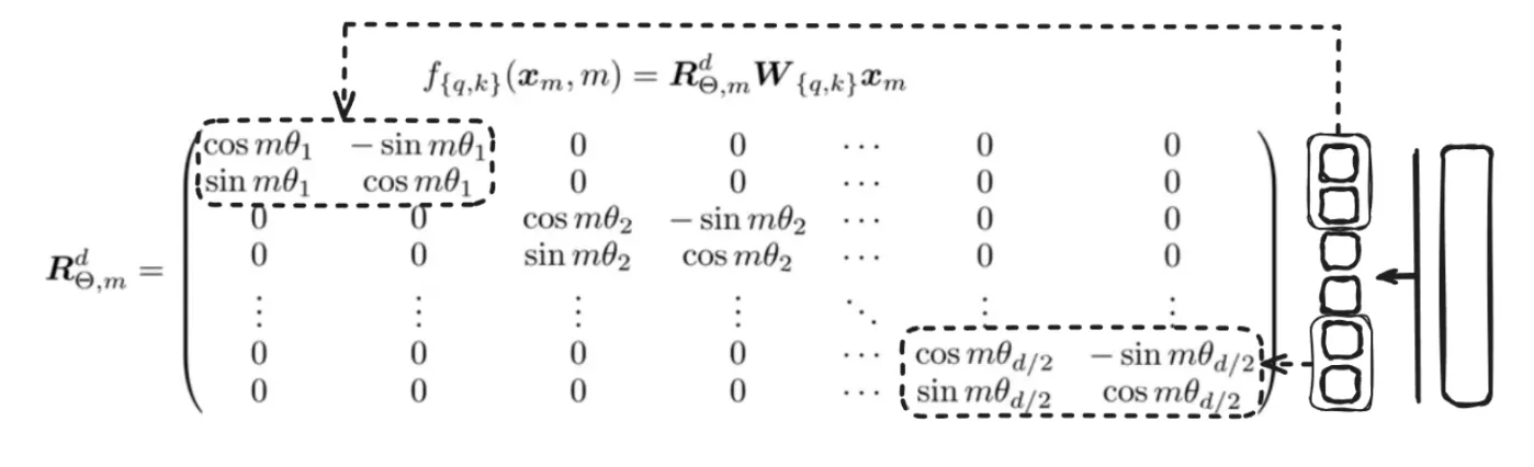
Here, the vector is divided into chunks of 2 and rotated by a certain m times θ.

But this kind of logic is really bad due to unnecessary memory and computation complexity. So, instead of this, we will implement using element-wise operations like this:

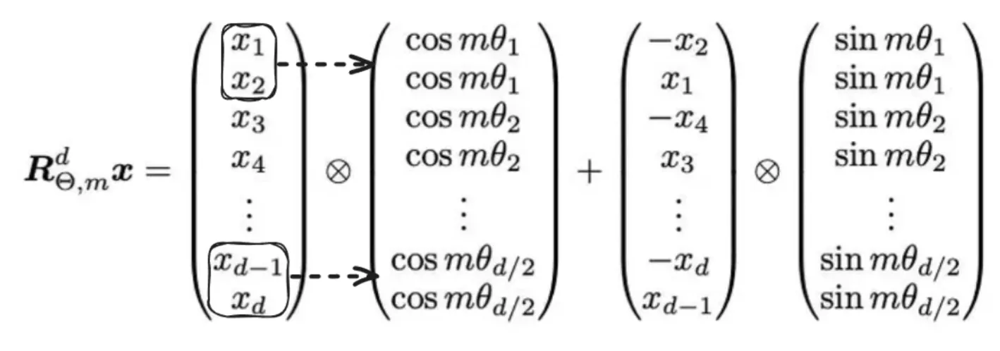
Normally, it is assumed that the dimension of the vector is even, which is normally the case, hence the assumption of making chunks of 2 here.

These Embeddings were utilised to train on several language models like BERT, RoFormer, etc., which showcased that these models trained faster with RoPE Embeddings over Sinusoidal Embeddings.

RoPE Components

RoPE has 2 types of components – High Frequency and Low Frequency components. High-frequency components are highly sensitive to positional changes. Low-frequency components, on the other hand, are less sensitive to relative positions, which allows transformers to maintain semantic attention over longer distances.

Therefore, the base N is increased from 10000 to 500000, which further slows down the low-frequency components, allowing the transformers to attend to relative tokens with large relative distance for capturing long-range dependencies.

But we need to understand how we can make sure RoPE can be utilised for longer context length sequences. Training a model directly on login context is very challenging due to training speed, memory footprint, and lack of large-scale data. These kinds of resources are very limited since only the top companies have this ability. We will also discuss longer context lengths in the next section, called Infini Attention, and their impact on the future of LLMs.

In short: One effective method is to rescale the position into the training context length; this is called position interpolation. This normally basically scales the position even further, slowing down the low-frequency components, hence allowing for longer context-length sequence information to be stored.

Infini Attention

Transformer models typically have limited-sized context windows. Infini Attention incorporates compressive memory into a vanilla attention mechanism and builds in both masked local attentions and long linear attention mechanisms in a single transformer block. Attention Mechanism comes with more disadvantages too, like:

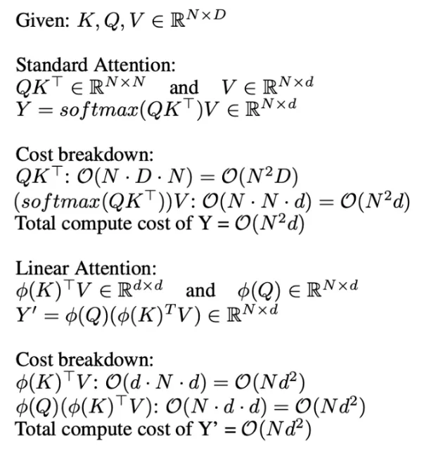
• It has quadratic complexity in both memory and computation time.
• Limitations in scaling the transformer to longer sequences (basically, learning a good representation from longer sequences becomes costly).

There were multiple experiments before the release of the “Leave No Context Behind: Efficient Infinite with Infini Attention”. Some techniques were like doing the computation row by row, by which we are trading off computation against memory, but still, we have quadratic complexity in computation, no matter how we distribute it. There were also attempts to do linear attention computations, which were also called linear attention or fast weights. Several approaches were made to get over this quadratic complexity bottleneck, but Infini Attention came ahead.

Compressive Memory

Infini Attention has a compressive memory unit in addition to the vanilla attention mechanism.

Compressive memory systems within Infini Attention are designed to efficiently handle long sequences by summarizing past information in a compact form. Instead of storing all past data, they maintain a fixed set of parameters that act as a summary of the sequence history. This summary can be updated over time and still retain useful information. The key idea is that whenever new information arrives, the memory is updated and its parameters are modified in such a way that the most relevant aspects of that new information are captured. This allows the model to recall important details later, without needing to store or process the entire sequence explicitly.

As a result, both the storage and computation requirements remain within a certain limit, making it much more scalable for processing long inputs, and hence a key player in shaping the future of LLMs.

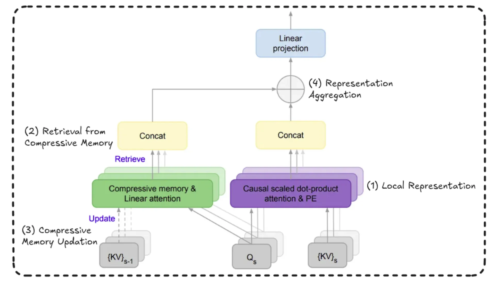
Very long sequences are broken into “s” segments. Each of these segments is processed by a causal attention mechanism, and a local representation is extracted from this current segment. Above this, another representation that has information about the sequence history is retrieved from compressed memory. Then, the current segment representation is appended or updated into the compressed memory. Finally, at the end, the local representation from the current segment and the retrieved information representation are combined to form a global long-range representation.

Basically, there are 4 main steps – Local Representation, Retrieval, Compressive Memory Update, and Representation Aggregation.

Complete Workflow

Within the larger context of understanding the future of LLMs, let’s first go over the complete workflow from the start, shall we?

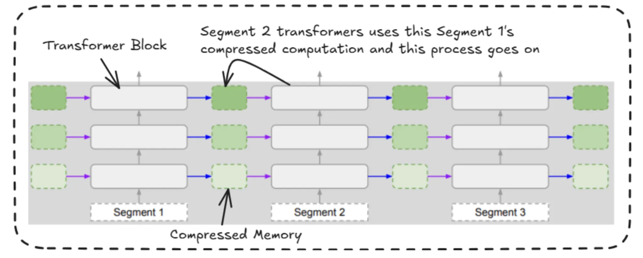
In Infini Attention, we divide the input sequence into multiple chunks or segments. For example, if the segment size is 100 tokens, we process those first 100 tokens as one segment using standard attention mechanisms. After computing the key-value pairs (attention outputs) for this segment, we store these representations in what’s called a compressive memory.

This memory acts as a bridge between segments. For each layer and each attention head, the model takes what it has learned from the current segment and adds it to this memory. Then, when the next segment is processed, it can access this memory, helping it retain information from earlier segments.

In short, local representations are still computed using standard attention, but Infini Attention enhances this by passing learned information forward through a shared memory structure.

This way of storing key value computations like queries into key transpose kind of computations into memory for the past time steps, and somehow be able to use it for future steps.

Now, we will see how this compressed memory is reused by the upcoming segments’ transformer blocks. So here we will be utilising the gating mechanism, which looks very similar to the logic used in LSTM’s gating mechanism.

Gating Mechanism

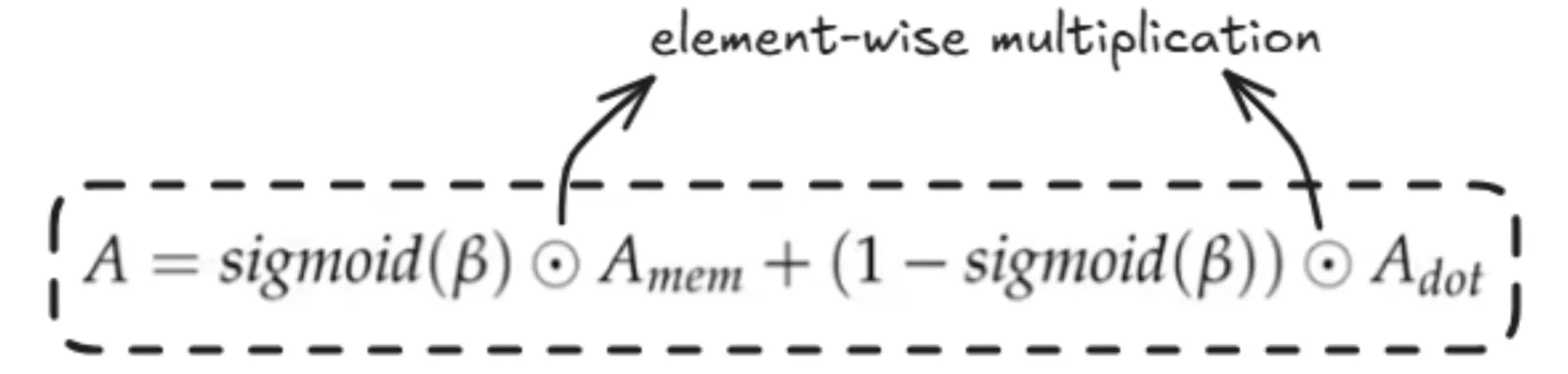
Here, we just don’t take the Q, K, V for current segment and essentially add positional embeddings(RoPE) and then compute the self attention as done above but also make use of information which we have from previous segments in the form of compressed memory by retrieving the info by using the the current Q (query) used to retrieve the information from the previous segments and the the current segment information is merged to get the overall attention value.

β here is called the gating scalar. It helps in the gated merging of the attention from current and previous segments. It is a learned parameter.

Now, we shall understand how this memory is obtained.

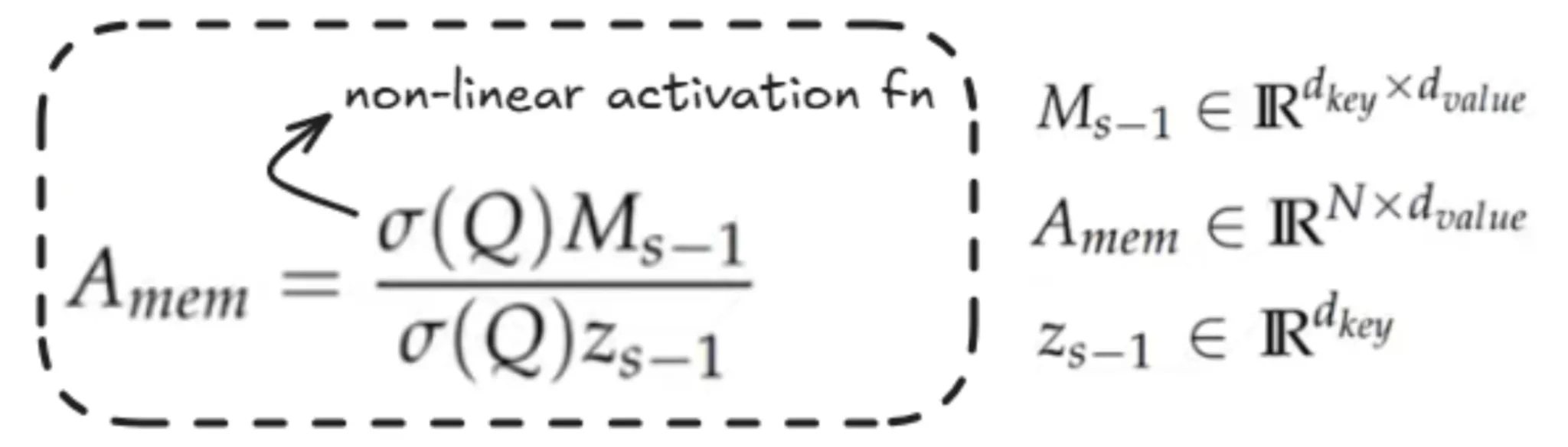
The information we have computed is stored in this matrix M, where in the numerator we utilise the Memory matrix of the previous segment. We take the current segment and apply an activation function, which here makes use of ELU.

Z here is the sum over all the keys. It doesn’t matter much; it is mostly used in this formula for normalisation purposes.

Now, let’s understand how memory is updated to compressed memory

Memory Update

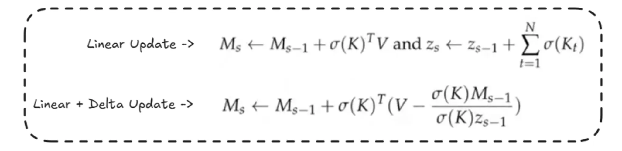
For the updation of memory, there are 2 methods:

1. Linear Update is simple, which sums the previous segment memory with the computation of the current segment.
2. In Linear + Delta updation, the computation of Z is similar to that in the above method, but here the memory updation is slightly different. Here, we subtract the contributions of some part of the memory. Basically, some attention computations have been done from previous segments, so we just update only the new knowledge, and the previous information is as it is. This helps in removing the duplicates and makes the memory less cluttered.

As for the retrieval part, we will be using the current segments Q (query) to retrieve the necessary memory fragments from the compressed memory and which is passed into the gating mechanism as explained above.

This is how the overall flow of Infini Attention works internally.
Let’s just look into some metrics on how effective Infini Attention is compared to other studies like Transformer XL, Reformer-based transformers, etc…

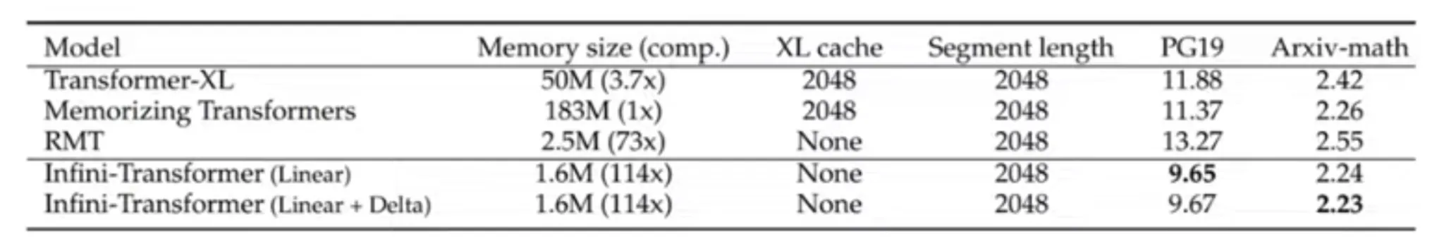
Here, the lower the score, the better the performance the model shows.

Another effective test was done about the retrieval task by experimenting with a zero-shot based passkey retrieval task where a numeric-based passkey is hidden with a huge context of textual information, and the transformer models were tasked to extract and retrieve these passkeys

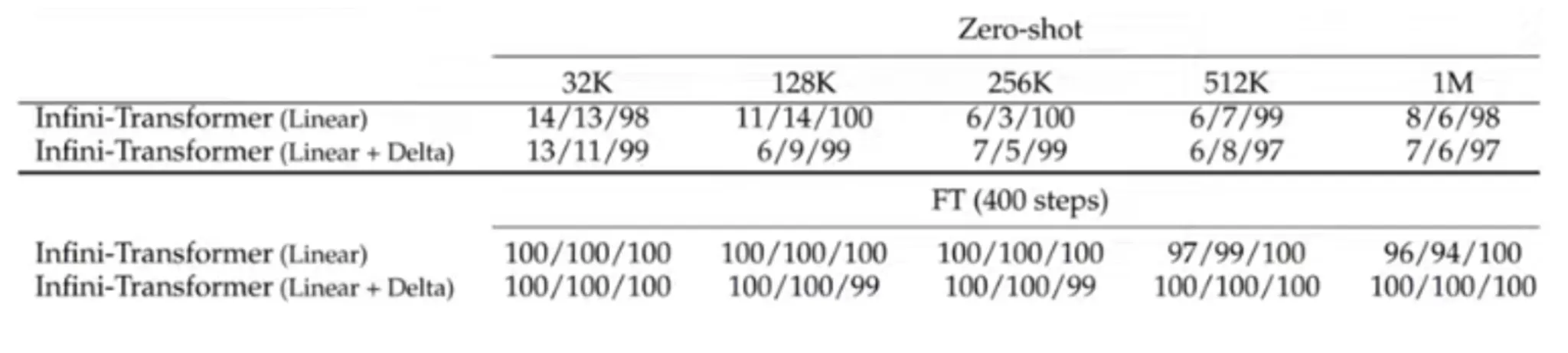
Here, we can see that Infini Transformer, which is finetuned up to 400 steps, is very effective at such retrieval tasks, especially when we use the Linear + Delta memory updation logic as explained above.

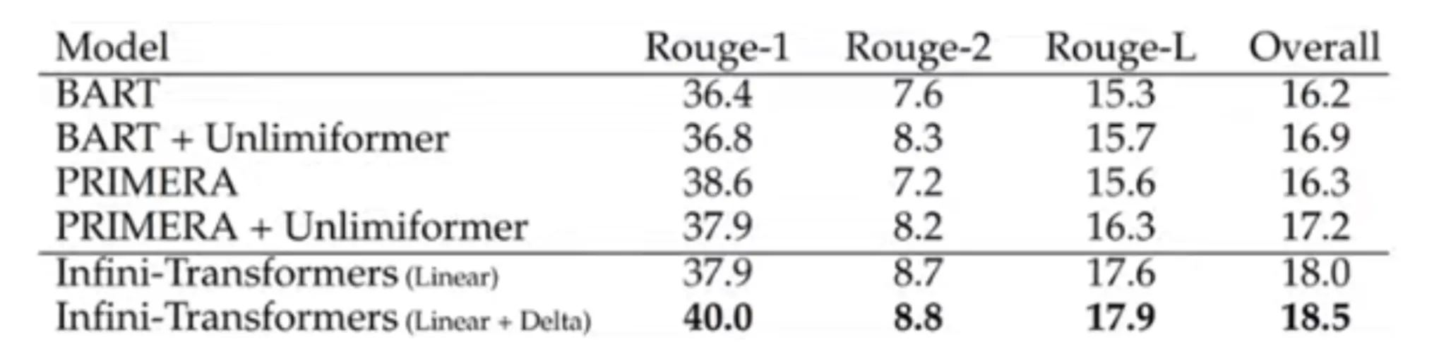
Infini Transformers perform better than several models like BART and PRIMERA when it comes to summarisation, as showcased with the provided ROUGE values in the above table. This gives us a key insight into the future of LLMs.

Conclusion

In this article, we explored three key innovations – Swish activation functions, RoPE embeddings, and Infini Attention that are actively shaping the next generation of large language models or the future of LLMs in general. Each of these advancements addresses critical limitations in previous architectures, whether it’s improving gradient flow, enhancing positional understanding, or extending context length efficiently.

As research in this field continues to accelerate, contributions from across the globe, fueled by a thriving open-source community, are allowing us to gain deeper insights into the internal workings of state-of-the-art LLMs, evolving them to new heights in the future. These breakthroughs are not only improving model performance but also redefining what’s possible in natural language understanding and generation.

The future of LLMs is being built on such foundational innovations, and staying updated on them is key to understanding where AI is headed next. You can read about how modern LLMs understand visual images here.