14 Powerful Techniques Defining the Evolution of Embedding

Summary:

• Evolution of Embeddings from basic count-based methods (TF-IDF, Word2Vec) to context-aware models like BERT and ELMo, which capture nuanced semantics by analyzing entire sentences bidirectionally.
• Leaderboards such as MTEB benchmark embeddings for tasks like retrieval and classification.
• Open-source platforms (Hugging Face) allow developers to access cutting-edge embeddings and deploy models tailored to different use cases.

You know how, back in the day, we used simple word‐count tricks to represent text? Well, things have come a long way since then. Now, when we talk about the evolution of embeddings, we mean numerical snapshots that capture not just which words appear but what they really mean, how they relate to each other in context, and even how they tie into images and other media. Embeddings power everything from search engines that understand your intent to recommendation systems that seem to read your mind. They’re at the heart of cutting‐edge AI and machine‐learning applications, too. So, let’s take a stroll through this evolution from raw counts to semantic vectors, exploring how each approach works, what it brings to the table, and where it falls short.

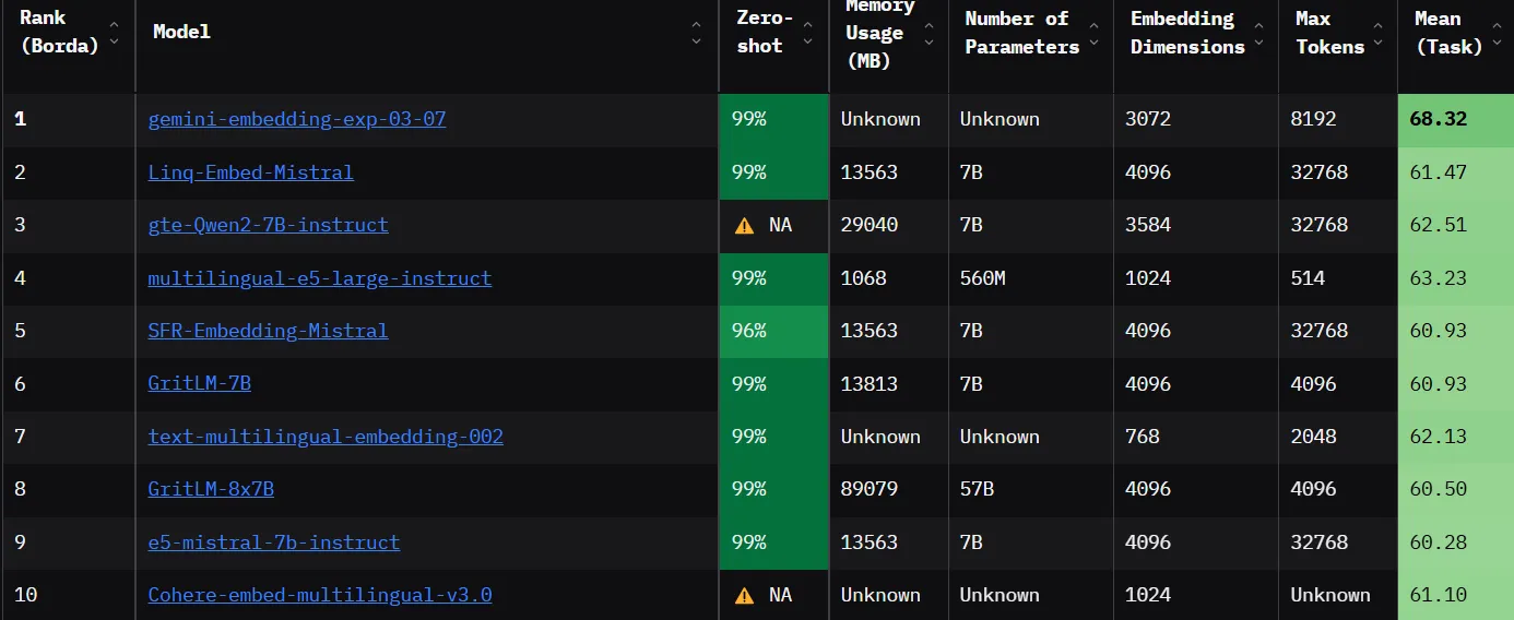
Ranking of Embeddings in MTEB Leaderboards

Most modern LLMs generate embeddings as intermediate outputs of their architectures. These can be extracted and fine-tuned for various downstream tasks, making LLM-based embeddings one of the most versatile tools available today.

To keep up with the fast-moving landscape, platforms like Hugging Face have introduced resources like the Massive Text Embedding Benchmark (MTEB) Leaderboard. This leaderboard ranks embedding models based on their performance across a wide range of tasks, including classification, clustering, retrieval, and more. This is substantially helping practitioners identify the best models for their use cases.

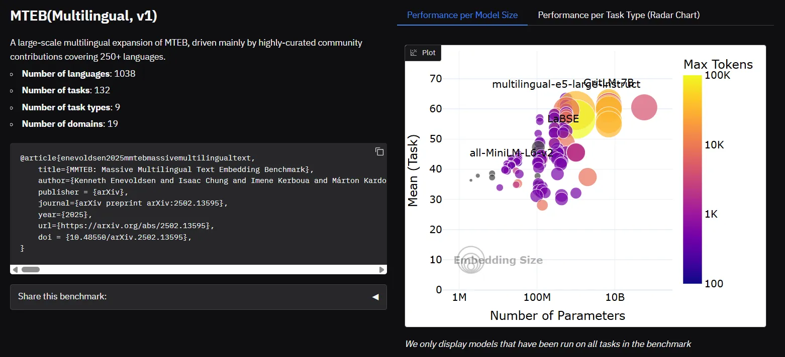
Armed with these leaderboard insights, let’s roll up our sleeves and dive into the vectorization toolbox – count vectors, TF–IDF, and other classic methods, which still serve as the essential building blocks for today’s sophisticated embeddings.

1. Count Vectorization

Count Vectorization is one of the simplest techniques for representing text. It emerged from the need to convert raw text into numerical form so that machine learning models could process it. In this method, each document is transformed into a vector that reflects the count of each word appearing in it. This straightforward approach laid the groundwork for more complex representations and is still useful in scenarios where interpretability is key.

How It Works

• Mechanism:
  • The text corpus is first tokenized into words. A vocabulary is built from all unique tokens.
  • Each document is represented as a vector where each dimension corresponds to the word’s respective vector in the vocabulary.
  • The value in each dimension is simply the frequency or count of a certain word in the document.
• Example: For a vocabulary [“apple“, “banana“, “cherry“], the document “apple apple cherry” becomes [2, 0, 1].
• Additional Detail: Count Vectorization serves as the foundation for many other approaches. Its simplicity does not capture any contextual or semantic information, but it remains an essential preprocessing step in many NLP pipelines.

Code Implementation

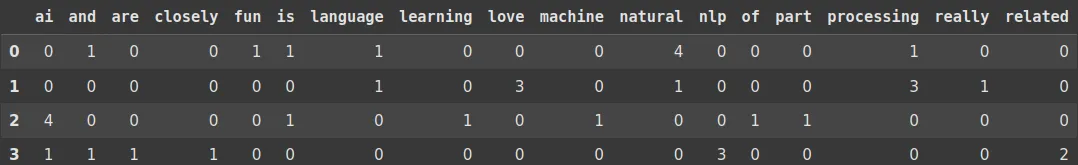
from sklearn.feature_extraction.text import CountVectorizer

import pandas as pd

# Sample text documents with repeated words

documents = [

	"Natural Language Processing is fun and natural natural natural",

	"I really love love love Natural Language Processing Processing Processing",

	"Machine Learning is a part of AI AI AI AI",

	"AI and NLP NLP NLP are closely related related"

]

# Initialize CountVectorizer

vectorizer = CountVectorizer()

# Fit and transform the text data

X = vectorizer.fit_transform(documents)

# Get feature names (unique words)

feature_names = vectorizer.get_feature_names_out()

# Convert to DataFrame for better visualization

df = pd.DataFrame(X.toarray(), columns=feature_names)

# Print the matrix

print(df)

Output:

Benefits

• Simplicity and Interpretability: Easy to implement and understand.
• Deterministic: Produces a fixed representation that is easy to analyze.

Shortcomings

• High Dimensionality and Sparsity: Vectors are often large and mostly zero, leading to inefficiencies.
• Lack of Semantic Context: Does not capture meaning or relationships between words.

2. One-Hot Encoding

One-hot encoding is one of the earliest approaches to representing words as vectors. Developed alongside early digital computing techniques in the 1950s and 1960s, it transforms categorical data, such as words, into binary vectors. Each word is represented uniquely, ensuring that no two words share similar representations, though this comes at the expense of capturing semantic similarity.

How It Works

• Mechanism:
  • Every word in the vocabulary is assigned a vector whose length equals the size of the vocabulary.
  • In each vector, all elements are 0 except for a single 1 in the position corresponding to that word.
• Example: With a vocabulary [“apple“, “banana“, “cherry“], the word “banana” is represented as [0, 1, 0].
• Additional Detail: One-hot vectors are completely orthogonal, which means that the cosine similarity between two different words is zero. This approach is simple and unambiguous but fails to capture any similarity (e.g., “apple” and “orange” appear equally dissimilar to “apple” and “car”).

Code Implementation

from sklearn.feature_extraction.text import CountVectorizer

import pandas as pd

# Sample text documents

documents = [

   "Natural Language Processing is fun and natural natural natural",

   "I really love love love Natural Language Processing Processing Processing",

   "Machine Learning is a part of AI AI AI AI",

   "AI and NLP NLP NLP are closely related related"

]

# Initialize CountVectorizer with binary=True for One-Hot Encoding

vectorizer = CountVectorizer(binary=True)

# Fit and transform the text data

X = vectorizer.fit_transform(documents)

# Get feature names (unique words)

feature_names = vectorizer.get_feature_names_out()

# Convert to DataFrame for better visualization

df = pd.DataFrame(X.toarray(), columns=feature_names)

# Print the one-hot encoded matrix

print(df)

Output:

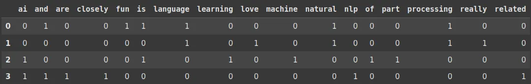
So, basically, you can view the difference between Count Vectorizer and One Hot Encoding. Count Vectorizer counts how many times a certain word exists in a sentence, whereas One Hot Encoding labels the word as 1 if it exists in a certain sentence/document.

When to Use What?

• Use CountVectorizer when the number of times a word appears is important (e.g., spam detection, document similarity).
• Use One-Hot Encoding when you only care about whether a word appears at least once (e.g., categorical feature encoding for ML models).

Benefits

• Clarity and Uniqueness: Each word has a distinct and non-overlapping representation
• Simplicity: Easy to implement with minimal computational overhead for small vocabularies.

Shortcomings

• Inefficiency with Large Vocabularies: Vectors become extremely high-dimensional and sparse.
• No Semantic Similarity: Does not allow for any relationships between words; all non-identical words are equally distant.

3. TF-IDF (Term Frequency-Inverse Document Frequency)

TF-IDF was developed to improve upon raw count methods by counting word occurrences and weighing words based on their overall importance in a corpus. Introduced in the early 1970s, TF-IDF is a cornerstone in information retrieval systems and text mining applications. It helps highlight terms that are significant in individual documents while downplaying words that are common across all documents.

How It Works

• Mechanism:
  • Term Frequency (TF): Measures how often a word appears in a document.
  • Inverse Document Frequency (IDF): Scales the importance of a word by considering how common or rare it is across all documents.
  • The final TF-IDF score is the product of TF and IDF.

• Example: Common words like “the” receive low scores, whereas more unique words receive higher scores, making them stand out in document analysis. Hence, we normally omit the frequent terms, which are also called Stopwords, in NLP tasks.
  
• Additional Detail: TF-IDF transforms raw frequency counts into a measure that can effectively differentiate between important keywords and commonly used words. It has become a standard method in search engines and document clustering.

Code Implementation

from sklearn.feature_extraction.text import TfidfVectorizer

import pandas as pd

import numpy as np

# Sample short sentences

documents = [

   "cat sits here",

   "dog barks loud",

   "cat barks loud"

]

# Initialize TfidfVectorizer to get both TF and IDF

vectorizer = TfidfVectorizer()

# Fit and transform the text data

X = vectorizer.fit_transform(documents)

# Extract feature names (unique words)

feature_names = vectorizer.get_feature_names_out()

# Get TF matrix (raw term frequencies)

tf_matrix = X.toarray()

# Compute IDF values manually

idf_values = vectorizer.idf_

# Compute TF-IDF manually (TF * IDF)

tfidf_matrix = tf_matrix * idf_values

# Convert to DataFrames for better visualization

df_tf = pd.DataFrame(tf_matrix, columns=feature_names)

df_idf = pd.DataFrame([idf_values], columns=feature_names)

df_tfidf = pd.DataFrame(tfidf_matrix, columns=feature_names)

# Print tables

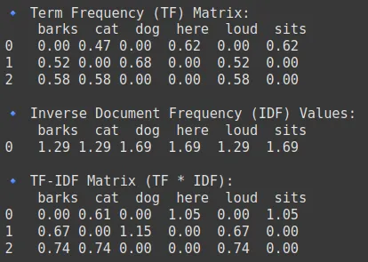
print("\n🔹 Term Frequency (TF) Matrix:\n", df_tf)

print("\n🔹 Inverse Document Frequency (IDF) Values:\n", df_idf)

print("\n🔹 TF-IDF Matrix (TF * IDF):\n", df_tfidf)

Output:

Benefits

• Enhanced Word Importance: Emphasizes content-specific words.
• Reduces Dimensionality: Filters out common words that add little value.

Shortcomings

• Sparse Representation: Despite weighting, the resulting vectors are still sparse.
• Lack of Context: Does not capture word order or deeper semantic relationships.

Also Read: Implementing Count Vectorizer and TF-IDF in NLP using PySpark

4. Okapi BM25

Okapi BM25, developed in the 1990s, is a probabilistic model designed primarily for ranking documents in information retrieval systems rather than as an embedding method per se. BM25 is an enhanced version of TF-IDF, commonly used in search engines and information retrieval. It improves upon TF-IDF by considering document length normalization and saturation of term frequency (i.e., diminishing returns for repeated words).

How It Works

• Mechanism:
  • Probabilistic Framework: This framework estimates the relevance of a document based on the frequency of query terms, adjusted by document length.
  • Uses parameters to control the influence of term frequency and to dampen the effect of very high counts.

Here we will be looking into the BM25 scoring mechanism:

BM25 introduces two parameters, k1 and b, which allow fine-tuning of the term frequency saturation and the length normalization, respectively. These parameters are crucial for optimizing the BM25 algorithm’s performance in various search contexts.

• Example: BM25 assigns higher relevance scores to documents that contain rare query terms with moderate frequency while adjusting for document length and vice versa.
  
• Additional Detail: Although BM25 does not produce vector embeddings, it has deeply influenced text retrieval systems by improving upon the shortcomings of TF-IDF in ranking documents.

Code Implementation

import numpy as np

import pandas as pd

from sklearn.feature_extraction.text import CountVectorizer

# Sample documents

documents = [

   "cat sits here",

   "dog barks loud",

   "cat barks loud"

]

# Compute Term Frequency (TF) using CountVectorizer

vectorizer = CountVectorizer()

X = vectorizer.fit_transform(documents)

tf_matrix = X.toarray()

feature_names = vectorizer.get_feature_names_out()

# Compute Inverse Document Frequency (IDF) for BM25

N = len(documents)  # Total number of documents

df = np.sum(tf_matrix > 0, axis=0)  # Document Frequency (DF) for each term

idf = np.log((N - df + 0.5) / (df + 0.5) + 1)  # BM25 IDF formula

# Compute BM25 scores

k1 = 1.5  # Smoothing parameter

b = 0.75  # Length normalization parameter

avgdl = np.mean([len(doc.split()) for doc in documents])  # Average document length

doc_lengths = np.array([len(doc.split()) for doc in documents])

bm25_matrix = np.zeros_like(tf_matrix, dtype=np.float64)

for i in range(N):  # For each document

   for j in range(len(feature_names)):  # For each term

       term_freq = tf_matrix[i, j]

       num = term_freq * (k1 + 1)

       denom = term_freq + k1 * (1 - b + b * (doc_lengths[i] / avgdl))

       bm25_matrix[i, j] = idf[j] * (num / denom)

# Convert to DataFrame for better visualization

df_tf = pd.DataFrame(tf_matrix, columns=feature_names)

df_idf = pd.DataFrame([idf], columns=feature_names)

df_bm25 = pd.DataFrame(bm25_matrix, columns=feature_names)

# Display the results

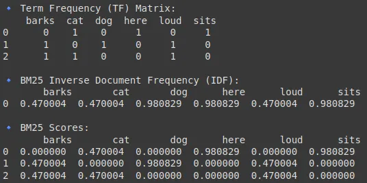
print("\n🔹 Term Frequency (TF) Matrix:\n", df_tf)

print("\n🔹 BM25 Inverse Document Frequency (IDF):\n", df_idf)

print("\n🔹 BM25 Scores:\n", df_bm25)

Output:

Code Implementation (Info Retrieval)

!pip install bm25s

import bm25s

# Create your corpus here

corpus = [

   "a cat is a feline and likes to purr",

   "a dog is the human's best friend and loves to play",

   "a bird is a beautiful animal that can fly",

   "a fish is a creature that lives in water and swims",

]

# Create the BM25 model and index the corpus

retriever = bm25s.BM25(corpus=corpus)

retriever.index(bm25s.tokenize(corpus))

# Query the corpus and get top-k results

query = "does the fish purr like a cat?"

results, scores = retriever.retrieve(bm25s.tokenize(query), k=2)

# Let's see what we got!

doc, score = results[0, 0], scores[0, 0]

print(f"Rank {i+1} (score: {score:.2f}): {doc}")

Output:

Benefits

• Improved Relevance Ranking: Better handles document length and term saturation.
• Widely Adopted: Standard in many modern search engines and IR systems.

Shortcomings

• Not a True Embedding: It scores documents rather than producing a continuous vector space representation.
• Parameter Sensitivity: Requires careful tuning for optimal performance.

Also Read: How to Create NLP Search Engine With BM25?

5. Word2Vec (CBOW and Skip-gram)

Introduced by Google in 2013, Word2Vec revolutionized NLP by learning dense, low-dimensional vector representations of words. It moved beyond counting and weighting by training shallow neural networks that capture semantic and syntactic relationships based on word context. Word2Vec comes in two flavors: Continuous Bag-of-Words (CBOW) and Skip-gram.

How It Works

• CBOW (Continuous Bag-of-Words):
  • Mechanism: Predicts a target word based on the surrounding context words.
  • Process: Takes multiple context words (ignoring the order) and learns to predict the central word.
• Skip-gram:
  • Mechanism: Uses the target word to predict its surrounding context words.
  • Process: Particularly effective for learning representations of rare words by focusing on their contexts.
    
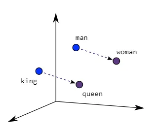
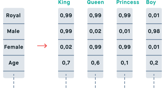
• Additional Detail: Both architectures use a neural network with one hidden layer and employ optimization tricks such as negative sampling or hierarchical softmax to manage computational complexity. The resulting embeddings capture nuanced semantic relationships for instance, “king” minus “man” plus “woman” approximates “queen.”

Code Implementation

!pip install numpy==1.24.3

from gensim.models import Word2Vec

import networkx as nx

import matplotlib.pyplot as plt

# Sample corpus

sentences = [

	["I", "love", "deep", "learning"],

	["Natural", "language", "processing", "is", "fun"],

	["Word2Vec", "is", "a", "great", "tool"],

	["AI", "is", "the", "future"],

]

# Train Word2Vec models

cbow_model = Word2Vec(sentences, vector_size=10, window=2, min_count=1, sg=0)  # CBOW

skipgram_model = Word2Vec(sentences, vector_size=10, window=2, min_count=1, sg=1)  # Skip-gram

# Get word vectors

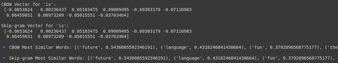
word = "is"

print(f"CBOW Vector for '{word}':\n", cbow_model.wv[word])

print(f"\nSkip-gram Vector for '{word}':\n", skipgram_model.wv[word])

# Get most similar words

print("\n🔹 CBOW Most Similar Words:", cbow_model.wv.most_similar(word))

print("\n🔹 Skip-gram Most Similar Words:", skipgram_model.wv.most_similar(word))

Output:

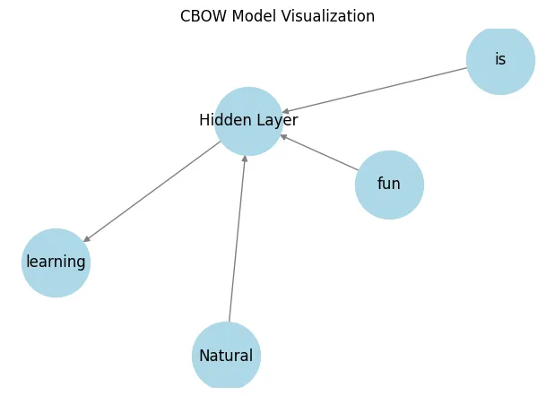
Visualizing the CBOW and Skip-gram:

def visualize_cbow():

   G = nx.DiGraph()

   # Nodes

   context_words = ["Natural", "is", "fun"]

   target_word = "learning"

   for word in context_words:

       G.add_edge(word, "Hidden Layer")

   G.add_edge("Hidden Layer", target_word)

   # Draw the network

   pos = nx.spring_layout(G)

   plt.figure(figsize=(6, 4))

   nx.draw(G, pos, with_labels=True, node_size=3000, node_color="lightblue", edge_color="gray")

   plt.title("CBOW Model Visualization")

   plt.show()

visualize_cbow()

Output:

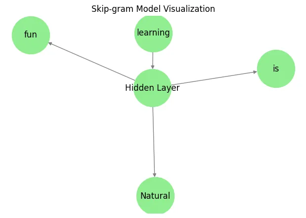
def visualize_skipgram():

   G = nx.DiGraph()

   # Nodes

   target_word = "learning"

   context_words = ["Natural", "is", "fun"]

   G.add_edge(target_word, "Hidden Layer")

   for word in context_words:

       G.add_edge("Hidden Layer", word)

   # Draw the network

   pos = nx.spring_layout(G)

   plt.figure(figsize=(6, 4))

   nx.draw(G, pos, with_labels=True, node_size=3000, node_color="lightgreen", edge_color="gray")

   plt.title("Skip-gram Model Visualization")

   plt.show()

visualize_skipgram()

Output:

Benefits

• Semantic Richness: Learns meaningful relationships between words.
• Efficient Training: Can be trained on large corpora relatively quickly.
• Dense Representations: Uses low-dimensional, continuous vectors that facilitate downstream processing.

Shortcomings

• Static Representations: Provides one embedding per word regardless of context.
• Context Limitations: Cannot disambiguate polysemous words that have different meanings in different contexts.

To read more about Word2Vec read this blog.

6. GloVe (Global Vectors for Word Representation)

GloVe, developed at Stanford in 2014, builds on the ideas of Word2Vec by combining global co-occurrence statistics with local context information. It was designed to produce word embeddings that capture overall corpus-level statistics, offering improved consistency across different contexts.

How It Works

• Mechanism:
  • Co-occurrence Matrix: Constructs a matrix capturing how frequently pairs of words appear together across the entire corpus.
    
    
    This logic of Co-occurence matrices are also widely used in Computer Vision too, especially under the topic of GLCM(Gray-Level Co-occurrence Matrix). It is a statistical method used in image processing and computer vision for texture analysis that considers the spatial relationship between pixels.
    
  • Matrix Factorization: Factorizes this matrix to derive word vectors that capture global statistical information.

• Additional Detail:
  Unlike Word2Vec’s purely predictive model, GloVe’s approach allows the model to learn the ratios of word co-occurrences, which some studies have found to be more robust in capturing semantic similarities and analogies.

Code Implementation

import numpy as np

# Load pre-trained GloVe embeddings

glove_model = api.load("glove-wiki-gigaword-50")  # You can use "glove-twitter-25", "glove-wiki-gigaword-100", etc.

# Example words

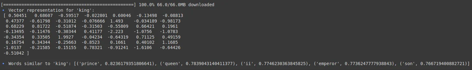
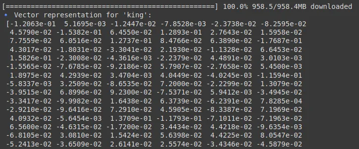
word = "king"

print(f"🔹 Vector representation for '{word}':\n", glove_model[word])

# Find similar words

similar_words = glove_model.most_similar(word, topn=5)

print("\n🔹 Words similar to 'king':", similar_words)

word1 = "king"

word2 = "queen"

similarity = glove_model.similarity(word1, word2)

print(f"🔹 Similarity between '{word1}' and '{word2}': {similarity:.4f}")

Output:

This image will help you understand how this similarity looks like when plotted:

Do refer to this for more in-depth information.

Benefits

• Global Context Integration: Uses entire corpus statistics to improve representation.
• Stability: Often yields more consistent embeddings across different contexts.

Shortcomings

• Resource Demanding: Building and factorizing large matrices can be computationally expensive.
• Static Nature: Similar to Word2Vec, it does not generate context-dependent embeddings.

GloVe learns embeddings from word co-occurrence matrices.

7. FastText

FastText, released by Facebook in 2016, extends Word2Vec by incorporating subword (character n-gram) information. This innovation helps the model handle rare words and morphologically rich languages by breaking words down into smaller units, thereby capturing internal structure.

How It Works

• Mechanism:
  • Subword Modeling: Represents each word as a sum of its character n-gram vectors.
  • Embedding Learning: Trains a model that uses these subword vectors to produce a final word embedding.
• Additional Detail:
  This method is particularly useful for languages with rich morphology and for dealing with out-of-vocabulary words. By decomposing words, FastText can generalize better across similar word forms and misspellings.

Code Implementation

import gensim.downloader as api

fasttext_model = api.load("fasttext-wiki-news-subwords-300")

# Example word

word = "king"

print(f"🔹 Vector representation for '{word}':\n", fasttext_model[word])

# Find similar words

similar_words = fasttext_model.most_similar(word, topn=5)

print("\n🔹 Words similar to 'king':", similar_words)

word1 = "king"

word2 = "queen"

similarity = fasttext_model.similarity(word1, word2)

print(f"🔹 Similarity between '{word1}' and '{word2}': {similarity:.4f}")

Output:

Benefits

• Handling OOV(Out of Vocabulary) Words: Improves performance when words are infrequent or unseen. Can say that the test dataset has some labels which do not exist in our train dataset.
• Morphological Awareness: Captures the internal structure of words.

Shortcomings

• Increased Complexity: The inclusion of subword information adds to computational overhead.
• Still Static or Fixed: Despite the improvements, FastText does not adjust embeddings based on a sentence’s surrounding context.

8. Doc2Vec

Doc2Vec extends Word2Vec’s ideas to larger bodies of text, such as sentences, paragraphs, or entire documents. Introduced in 2014, it provides a means to obtain fixed-length vector representations for variable-length texts, enabling more effective document classification, clustering, and retrieval.

How It Works

• Mechanism:
  • Distributed Memory (DM) Model: Augments the Word2Vec architecture by adding a unique document vector that, along with context words, predicts a target word.
  • Distributed Bag-of-Words (DBOW) Model: Learns document vectors by predicting words randomly sampled from the document.
• Additional Detail:
  These models learn document-level embeddings that capture the overall semantic content of the text. They are especially useful for tasks where the structure and theme of the entire document are important.

Code Implementation

import gensim

from gensim.models.doc2vec import Doc2Vec, TaggedDocument

import nltk

nltk.download('punkt_tab')

# Sample documents

documents = [

	"Machine learning is amazing",

	"Natural language processing enables AI to understand text",

	"Deep learning advances artificial intelligence",

	"Word embeddings improve NLP tasks",

	"Doc2Vec is an extension of Word2Vec"

]

# Tokenize and tag documents

tagged_data = [TaggedDocument(words=nltk.word_tokenize(doc.lower()), tags=[str(i)]) for i, doc in enumerate(documents)]

# Print tagged data

print(tagged_data)

# Define model parameters

model = Doc2Vec(vector_size=50, window=2, min_count=1, workers=4, epochs=100)

# Build vocabulary

model.build_vocab(tagged_data)

# Train the model

model.train(tagged_data, total_examples=model.corpus_count, epochs=model.epochs)

# Test a document by generating its vector

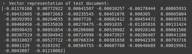
test_doc = "Artificial intelligence uses machine learning"

test_vector = model.infer_vector(nltk.word_tokenize(test_doc.lower()))

print(f"🔹 Vector representation of test document:\n{test_vector}")

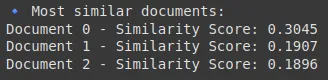
# Find most similar documents to the test document

similar_docs = model.dv.most_similar([test_vector], topn=3)

print("🔹 Most similar documents:")

for tag, score in similar_docs:

	print(f"Document {tag} - Similarity Score: {score:.4f}")

Output:

Benefits

• Document-Level Representation: Effectively captures thematic and contextual information of larger texts.
• Versatility: Useful in a variety of tasks, from recommendation systems to clustering and summarization.

Shortcomings

• Training Sensitivity: Requires significant data and careful tuning to produce high-quality docent vectors.
• Static Embeddings: Each document is represented by one vector regardless of the internal variability of content.

9. InferSent

InferSent, developed by Facebook in 2017, was designed to generate high-quality sentence embeddings through supervised learning on natural language inference (NLI) datasets. It aims to capture semantic nuances at the sentence level, making it highly effective for tasks like semantic similarity and textual entailment.

How It Works

• Mechanism:
  • Supervised Training: Uses labeled NLI data to learn sentence representations that reflect the logical relationships between sentences.
  • Bidirectional LSTMs: Employs recurrent neural networks that process sentences from both directions to capture context.
• Additional Detail:
  The model leverages supervised understanding to refine embeddings so that semantically similar sentences are closer together in the vector space, greatly enhancing performance on tasks like sentiment analysis and paraphrase detection.

Code Implementation

You can follow this Kaggle Notebook to implement this.

Output:

Benefits

• Rich Semantic Capturing: Provides deep, contextually nuanced sentence representations.
• Task-Optimized: Excels at capturing relationships required for semantic inference tasks.

Shortcomings

• Dependence on Labeled Data: Requires extensively annotated datasets for training.
• Computationally Intensive: More resource-demanding than unsupervised methods.

10. Universal Sentence Encoder (USE)

The Universal Sentence Encoder (USE) is a model developed by Google to create high-quality, general-purpose sentence embeddings. Released in 2018, USE has been designed to work well across a variety of NLP tasks with minimal fine-tuning, making it a versatile tool for applications ranging from semantic search to text classification.

How It Works

• Mechanism:
  • Architecture Options: USE can be implemented using Transformer architectures or Deep Averaging Networks (DANs) to encode sentences.
  • Pretraining: Trained on large, diverse datasets to capture broad language patterns, it maps sentences into a fixed-dimensional space.
• Additional Detail:
  USE provides robust embeddings across domains and tasks, making it an excellent “out-of-the-box” solution. Its design balances performance and efficiency, offering high-level embeddings without the need for extensive task-specific tuning.

Code Implementation

import tensorflow_hub as hub

import tensorflow as tf

import numpy as np

# Load the model (this may take a few seconds on first run)

embed = hub.load("https://tfhub.dev/google/universal-sentence-encoder/4")

print("✅ USE model loaded successfully!")

# Sample sentences

sentences = [

	"Machine learning is fun.",

	"Artificial intelligence and machine learning are related.",

	"I love playing football.",

	"Deep learning is a subset of machine learning."

]

# Get sentence embeddings

embeddings = embed(sentences)

# Convert to NumPy for easier manipulation

embeddings_np = embeddings.numpy()

# Display shape and first vector

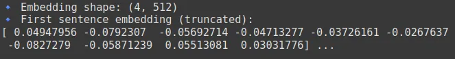
print(f"🔹 Embedding shape: {embeddings_np.shape}")

print(f"🔹 First sentence embedding (truncated):\n{embeddings_np[0][:10]} ...")

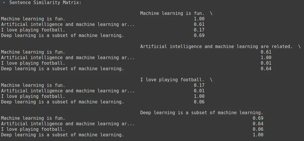
from sklearn.metrics.pairwise import cosine_similarity

# Compute pairwise cosine similarities

similarity_matrix = cosine_similarity(embeddings_np)

# Display similarity matrix

import pandas as pd

similarity_df = pd.DataFrame(similarity_matrix, index=sentences, columns=sentences)

print("🔹 Sentence Similarity Matrix:\n")

print(similarity_df.round(2))

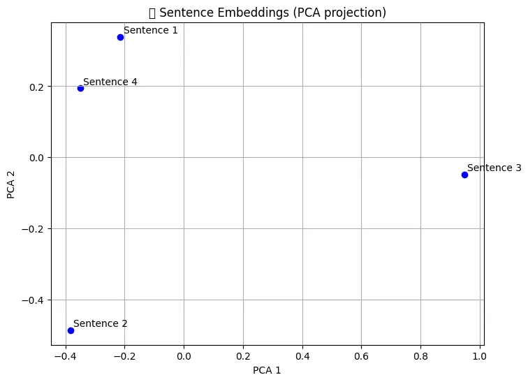
import matplotlib.pyplot as plt

from sklearn.decomposition import PCA

# Reduce to 2D

pca = PCA(n_components=2)

reduced = pca.fit_transform(embeddings_np)

# Plot

plt.figure(figsize=(8, 6))

plt.scatter(reduced[:, 0], reduced[:, 1], color='blue')

for i, sentence in enumerate(sentences):

	plt.annotate(f"Sentence {i+1}", (reduced[i, 0]+0.01, reduced[i, 1]+0.01))

plt.title("📊 Sentence Embeddings (PCA projection)")

plt.xlabel("PCA 1")

plt.ylabel("PCA 2")

plt.grid(True)

plt.show()

Output:

Benefits

• Versatility: Well-suited for a broad range of applications without additional training.
• Pretrained Convenience: Ready for immediate use, saving time and computational resources.

Shortcomings

• Fixed Representations: Produces a single embedding per sentence without dynamically adjusting to different contexts.
• Model Size: Some variants are quite large, which can affect deployment in resource-limited environments.

11. Node2Vec

Node2Vec is a method originally designed for learning node embeddings in graph structures. While not a text representation method per se, it is increasingly applied in NLP tasks that involve network or graph data, such as social networks or knowledge graphs. Introduced around 2016, it helps capture structural relationships in graph data.

Use Cases: Node classification, link prediction, graph clustering, recommendation systems.

How It Works

• Mechanism:
  • Random Walks: Performs biased random walks on a graph to generate sequences of nodes.
  • Skip-gram Model: Applies a strategy similar to Word2Vec on these sequences to learn low-dimensional embeddings for nodes.
• Additional Detail:
  By simulating the sentences within the nodes, Node2Vec effectively captures the local and global structure of the graphs. It is highly adaptive and can be used for various downstream tasks, such as clustering, classification or recommendation systems in networked data.

Code Implementation

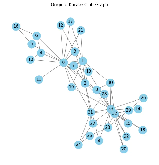
We will use this ready-made graph from NetworkX to view our Node2Vec implementation.To learn more about the Karate Club Graph, click here.

!pip install numpy==1.24.3 # Adjust version if needed

import networkx as nx

import numpy as np

from node2vec import Node2Vec

import matplotlib.pyplot as plt

from sklearn.decomposition import PCA

# Create a simple graph

G = nx.karate_club_graph()  # A famous test graph with 34 nodes

# Visualize original graph

plt.figure(figsize=(6, 6))

nx.draw(G, with_labels=True, node_color='skyblue', edge_color='gray', node_size=500)

plt.title("Original Karate Club Graph")

plt.show()

# Initialize Node2Vec model

node2vec = Node2Vec(G, dimensions=64, walk_length=30, num_walks=200, workers=2)

# Train the model (Word2Vec under the hood)

model = node2vec.fit(window=10, min_count=1, batch_words=4)

# Get the vector for a specific node

node_id = 0

vector = model.wv[str(node_id)]  # Note: Node IDs are stored as strings

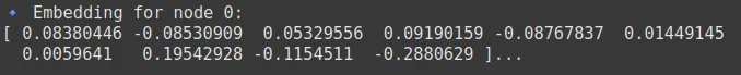
print(f"🔹 Embedding for node {node_id}:\n{vector[:10]}...")  # Truncated

# Get all embeddings

node_ids = model.wv.index_to_key

embeddings = np.array([model.wv[node] for node in node_ids])

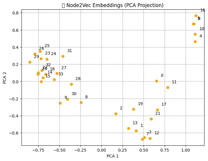
# Reduce dimensions to 2D

pca = PCA(n_components=2)

reduced = pca.fit_transform(embeddings)

# Plot embeddings

plt.figure(figsize=(8, 6))

plt.scatter(reduced[:, 0], reduced[:, 1], color='orange')

for i, node in enumerate(node_ids):

	plt.annotate(node, (reduced[i, 0] + 0.05, reduced[i, 1] + 0.05))

plt.title("📊 Node2Vec Embeddings (PCA Projection)")

plt.xlabel("PCA 1")

plt.ylabel("PCA 2")

plt.grid(True)

plt.show()

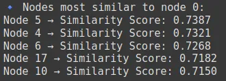
# Find most similar nodes to node 0

similar_nodes = model.wv.most_similar(str(0), topn=5)

print("🔹 Nodes most similar to node 0:")

for node, score in similar_nodes:

	print(f"Node {node} → Similarity Score: {score:.4f}")

Output:

Benefits

• Graph Structure Capture: Excels at embedding nodes with rich relational information.
• Flexibility: Can be applied to any graph-structured data, not just language.

Shortcomings

• Domain Specificity: Less applicable to plain text unless represented as a graph.
• Parameter Sensitivity: The quality of embeddings is sensitive to the parameters used in random walks.

12. ELMo (Embeddings from Language Models)

ELMo, introduced by the Allen Institute for AI in 2018, marked a breakthrough by providing deep contextualized word representations. Unlike earlier models that generate a single vector per word, ELMo produces dynamic embeddings that change based on a sentence’s context, capturing both syntactic and semantic nuances.

How It Works

• Mechanism:
  • Bidirectional LSTMs: Processes text in both forward and backward directions to capture full contextual information.
  • Layered Representations: Combines representations from multiple layers of the neural network, each capturing different aspects of language.
• Additional Detail:
  The key innovation is that the same word can have different embeddings depending on its usage, allowing ELMo to handle ambiguity and polysemy more effectively. This context sensitivity leads to improvements in many downstream NLP tasks. It operates through customizable parameters, including dimensions (embedding vector size), walk_length (nodes per random walk), num_walks (walks per node), and bias parameters p (return factor) and q (in-out factor) that control walk behavior by balancing breadth-first (BFS) and depth-first (DFS) search tendencies. The methodology combines biased random walks, which explore node neighborhoods with tunable search strategies, with Word2Vec’s Skip-gram architecture to learn embeddings preserving network structure and node relationships. Node2Vec enables effective node classification, link prediction, and graph clustering by capturing both local network patterns and broader structures in the embedding space.

Code Implementation

To implement and understand more about ELMo, you can refer to this article here.

Benefits

• Context-Awareness: Provides word embeddings that vary in accordance with the context.
• Enhanced Performance: Improves results based on a variety of tasks, including sentiment analysis, question answering, and machine translation.

Shortcomings

• Computationally Demanding: Requires more resources for training and inference.
• Complex Architecture: Challenging to implement and fine-tune compared to other simpler models.

13. BERT and Its Variants

What is BERT?

BERT or Bidirectional Encoder Representations from Transformers, released by Google in 2018, revolutionized NLP by introducing a transformer-based architecture that captures bidirectional context. Unlike previous models that processed text in a unidirectional manner, BERT considers both the left and right context of each word. This deep, contextual understanding enables BERT to excel at tasks ranging from question answering and sentiment analysis to named entity recognition.

How It Works:

• Transformer Architecture: BERT is built on a multi-layer transformer network that uses a self-attention mechanism to capture dependencies between all words in a sentence simultaneously. This allows the model to weigh the dependency of each word on every other word.
• Masked Language Modeling: During pre-training, BERT randomly masks certain words in the input and then predicts them based on their context. This forces the model to learn bidirectional context and develop a robust understanding of language patterns.
• Next Sentence Prediction: BERT is also trained on pairs of sentences, learning to predict whether one sentence logically follows another. This helps it capture relationships between sentences, an essential feature for tasks like document classification and natural language inference.

Additional Detail: BERT’s architecture allows it to learn intricate patterns of language, including syntax and semantics. Fine-tuning on downstream tasks is straightforward, leading to state-of-the-art performance across many benchmarks.

Benefits:

• Deep Contextual Understanding: By considering both past and future context, BERT generates richer, more nuanced word representations.
• Versatility: BERT can be fine-tuned with relatively little additional training for a wide range of downstream tasks.

Shortcomings:

• Heavy Computational Load: The model requires significant computational resources during both training and inference.
• Large Model Size: BERT’s large number of parameters can make it challenging to deploy in resource-constrained environments.

SBERT (Sentence-BERT)

Sentence-BERT (SBERT) was introduced in 2019 to address a key limitation of BERT—its inefficiency in generating semantically meaningful sentence embeddings for tasks like semantic similarity, clustering, and information retrieval. SBERT adapts BERT’s architecture to produce fixed-size sentence embeddings that are optimized for comparing the meaning of sentences directly.

How It Works:

• Siamese Network Architecture: SBERT modifies the original BERT structure by employing a siamese (or triplet) network architecture. This means it processes two (or more) sentences in parallel through identical BERT-based encoders, allowing the model to learn embeddings such that semantically similar sentences are close together in vector space.
• Pooling Operation: After processing sentences through BERT, SBERT applies a pooling strategy (commonly meaning pooling) on the token embeddings to produce a fixed-size vector for each sentence.
• Fine-Tuning with Sentence Pairs: SBERT is fine-tuned on tasks involving sentence pairs using contrastive or triplet loss. This training objective encourages the model to place similar sentences closer together and dissimilar ones further apart in the embedding space.

Benefits:

• Efficient Sentence Comparisons: SBERT is optimized for tasks like semantic search and clustering. Due to its fixed size and semantically rich sentence embeddings, comparing tens of thousands of sentences becomes computationally feasible.
• Versatility in Downstream Tasks: SBERT embeddings are effective for a variety of applications, such as paraphrase detection, semantic textual similarity, and information retrieval.

Shortcomings:

• Dependence on Fine-Tuning Data: The quality of SBERT embeddings can be heavily influenced by the domain and quality of the training data used during fine-tuning.
• Resource Intensive Training: Although inference is efficient, the initial fine-tuning process requires considerable computational resources.

DistilBERT

DistilBERT, introduced by Hugging Face in 2019, is a lighter and faster variant of BERT that retains much of its performance. It was created using a technique called knowledge distillation, where a smaller model (student) is trained to mimic the behavior of a larger, pre-trained model (teacher), in this case, BERT.

How It Works:

• Knowledge Distillation: DistilBERT is trained to match the output distributions of the original BERT model while using fewer parameters. It removes some layers (e.g., 6 instead of 12 in the BERT-base) but maintains crucial learning behavior.
• Loss Function: The training uses a combination of language modeling loss and distillation loss (KL divergence between teacher and student logits).
• Speed Optimization: DistilBERT is optimized to be 60% faster during inference while retaining ~97% of BERT’s performance on downstream tasks.

Benefits:

• Lightweight and Fast: Ideal for real-time or mobile applications due to reduced computational demands.
• Competitive Performance: Achieves near-BERT accuracy with significantly lower resource usage.

Shortcomings:

• Slight Drop in Accuracy: While very close, it might slightly underperform compared to the full BERT model in complex tasks.
• Limited Fine-Tuning Flexibility: It may not generalize as well in niche domains as full-sized models.

RoBERTa

RoBERTa or Robustly Optimized BERT Pretraining Approach was introduced by Facebook AI in 2019 as a robust enhancement over BERT. It tweaks the pretraining methodology to improve performance significantly across a wide range of tasks.

How It Works:

• Training Enhancements:
  • Removes the Next Sentence Prediction (NSP) objective, which was found to hurt performance in some settings.
  • Trains on much larger datasets (e.g., Common Crawl) and for longer durations.
  • Uses larger mini-batches and more training steps to stabilize and optimize learning.
• Dynamic Masking: This method applies masking on the fly during each training epoch, exposing the model to more diverse masking patterns than BERT’s static masking.

Benefits:

• Superior Performance: Outperforms BERT on several benchmarks, including GLUE and SQuAD.
• Robust Learning: Better generalization across domains due to improved training data and strategies.

Shortcomings:

• Resource Intensive: Even more computationally demanding than BERT.
• Overfitting Risk: With extensive training and large datasets, there’s a risk of overfitting if not handled carefully.

Code Implementation

from transformers import AutoTokenizer, AutoModel

import torch

# Input sentence for embedding

sentence = "Natural Language Processing is transforming how machines understand humans."

# Choose device (GPU if available)

device = torch.device("cuda" if torch.cuda.is_available() else "cpu")

# =============================

# 1. BERT Base Uncased

# =============================

# model_name = "bert-base-uncased"

# =============================

# 2. SBERT - Sentence-BERT

# =============================

# model_name = "sentence-transformers/all-MiniLM-L6-v2"

# =============================

# 3. DistilBERT

# =============================

# model_name = "distilbert-base-uncased"

# =============================

# 4. RoBERTa

# =============================

model_name = "roberta-base"  # Only RoBERTa is active now uncomment other to test other models

# Load tokenizer and model

tokenizer = AutoTokenizer.from_pretrained(model_name)

model = AutoModel.from_pretrained(model_name).to(device)

model.eval()

# Tokenize input

inputs = tokenizer(sentence, return_tensors='pt', truncation=True, padding=True).to(device)

# Forward pass to get embeddings

with torch.no_grad():

    outputs = model(**inputs)

# Get token embeddings

token_embeddings = outputs.last_hidden_state  # (batch_size, seq_len, hidden_size)

# Mean Pooling for sentence embedding

sentence_embedding = torch.mean(token_embeddings, dim=1)

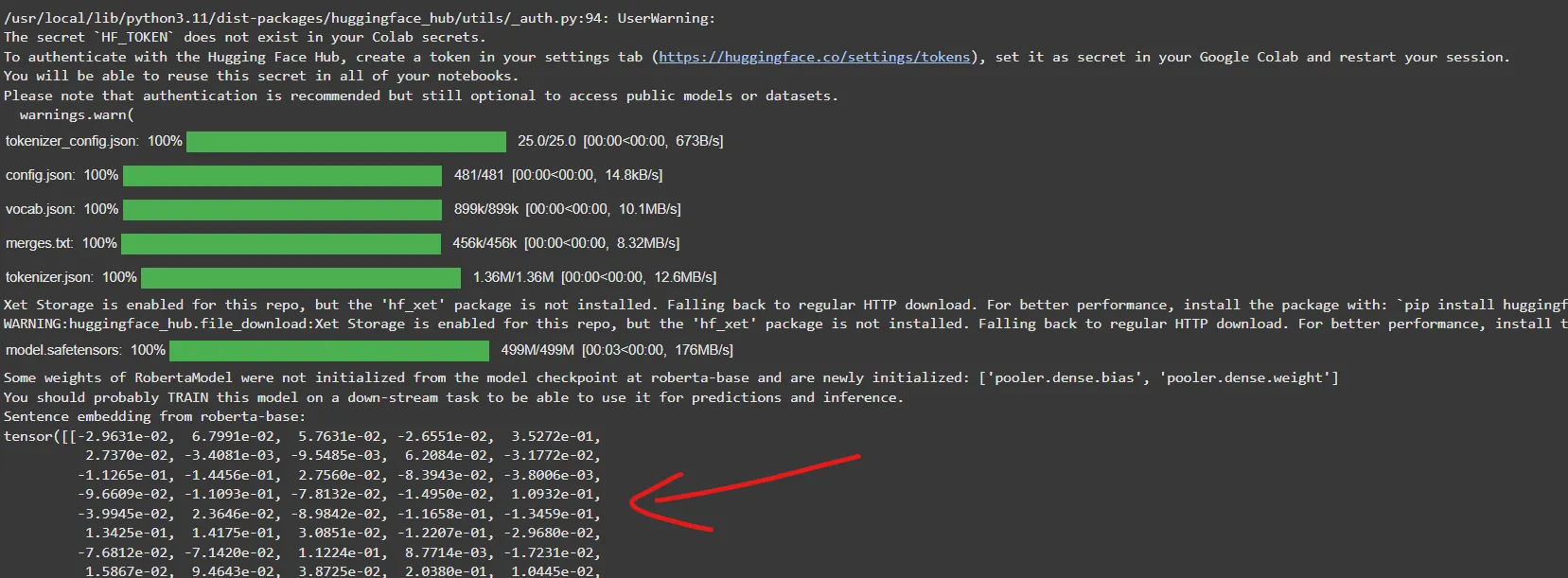
print(f"Sentence embedding from {model_name}:")

print(sentence_embedding)

Output:

Summary

• BERT provides deep, bidirectional contextualized embeddings ideal for a wide range of NLP tasks. It captures intricate language patterns through transformer-based self-attention but produces token-level embeddings that need to be aggregated for sentence-level tasks.
• SBERT extends BERT by transforming it into a model that directly produces meaningful sentence embeddings. With its siamese network architecture and contrastive learning objectives, SBERT excels at tasks requiring fast and accurate semantic comparisons between sentences, such as semantic search, paraphrase detection, and sentence clustering.
• DistilBERT offers a lighter, faster alternative to BERT by using knowledge distillation. It retains most of BERT’s performance while being more suitable for real-time or resource-constrained applications. It is ideal when inference speed and efficiency are key concerns, though it may slightly underperform in complex scenarios.
• RoBERTa improves upon BERT by modifying its pre-training regime, removing the next sentence prediction task by using larger datasets, and applying dynamic masking. These changes result in better generalization and performance across benchmarks, though at the cost of increased computational resources.

Other Notable BERT Variants

While BERT and its direct descendants like SBERT, DistilBERT, and RoBERTa have made a significant impact in NLP, several other powerful variants have emerged to address different limitations and enhance specific capabilities:

• ALBERT (A Lite BERT)
  ALBERT is a more efficient version of BERT that reduces the number of parameters through two key innovations: factorized embedding parameterization (which separates the size of the vocabulary embedding from the hidden layers) and cross-layer parameter sharing (which reuses weights across transformer layers). These changes make ALBERT faster and more memory-efficient while preserving performance on many NLP benchmarks.
  
• XLNet
  Unlike BERT, which relies on masked language modeling, XLNet adopts a permutation-based autoregressive training strategy. This allows it to capture bidirectional context without relying on data corruption like masking. XLNet also integrates ideas from Transformer-XL, which enables it to model longer-term dependencies and outperform BERT on several NLP tasks.
  
• T5 (Text-to-Text Transfer Transformer)
  Developed by Google Research, T5 frames every NLP task, from translation to classification, as a text-to-text problem. For example, instead of producing a classification label directly, T5 learns to generate the label as a word or phrase. This unified approach makes it highly flexible and powerful, capable of tackling a broad spectrum of NLP challenges.

14. CLIP and BLIP

Modern multimodal models like CLIP (Contrastive Language-Image Pretraining) and BLIP (Bootstrapping Language-Image Pre-training) represent the latest frontier in embedding techniques. They bridge the gap between textual and visual data, enabling tasks that involve both language and images. These models have become essential for applications such as image search, captioning, and visual question answering.

How It Works

• CLIP:
  • Mechanism: Trains on large datasets of image-text pairs, using contrastive learning to align image embeddings with corresponding text embeddings.
  • Process: The model learns to map images and text into a shared vector space where related pairs are closer together.
• BLIP:
  • Mechanism: Uses a bootstrapping approach to refine the alignment between language and vision through iterative training.
  • Process: Improves upon initial alignments to achieve more accurate multimodal representations.
• Additional Detail:
  These models harness the power of transformers for text and convolutional or transformer-based networks for images. Their ability to jointly reason about text and visual content has opened up new possibilities in multimodal AI research.

Code Implementation

from transformers import CLIPProcessor, CLIPModel

# from transformers import BlipProcessor, BlipModel  # Uncomment to use BLIP

from PIL import Image

import torch

import requests

# Choose device

device = torch.device("cuda" if torch.cuda.is_available() else "cpu")

# Load a sample image and text

image_url = "https://huggingface.co/datasets/huggingface/documentation-images/resolve/main/datasets/cat_style_layout.png"

image = Image.open(requests.get(image_url, stream=True).raw).convert("RGB")

text = "a cute puppy"

# ===========================

# 1. CLIP (for Embeddings)

# ===========================

clip_model_name = "openai/clip-vit-base-patch32"

clip_model = CLIPModel.from_pretrained(clip_model_name).to(device)

clip_processor = CLIPProcessor.from_pretrained(clip_model_name)

# Preprocess input

inputs = clip_processor(text=[text], images=image, return_tensors="pt", padding=True).to(device)

# Get text and image embeddings

with torch.no_grad():

    text_embeddings = clip_model.get_text_features(input_ids=inputs["input_ids"])

    image_embeddings = clip_model.get_image_features(pixel_values=inputs["pixel_values"])

# Normalize embeddings (optional)

text_embeddings = text_embeddings / text_embeddings.norm(dim=-1, keepdim=True)

image_embeddings = image_embeddings / image_embeddings.norm(dim=-1, keepdim=True)

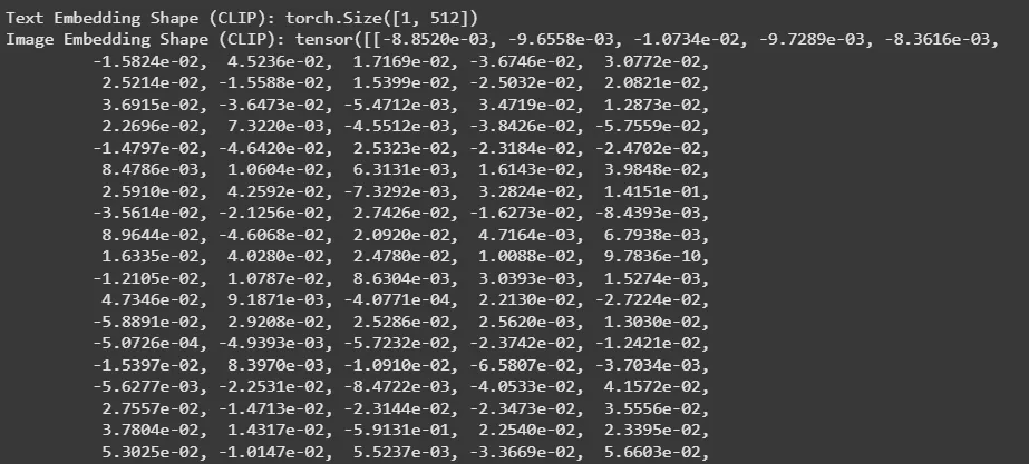
print("Text Embedding Shape (CLIP):", text_embeddings.shape)

print("Image Embedding Shape (CLIP):", image_embeddings)

# ===========================

# 2. BLIP (commented)

# ===========================

# blip_model_name = "Salesforce/blip-image-text-matching-base"

# blip_processor = BlipProcessor.from_pretrained(blip_model_name)

# blip_model = BlipModel.from_pretrained(blip_model_name).to(device)

# inputs = blip_processor(images=image, text=text, return_tensors="pt").to(device)

# with torch.no_grad():

#     text_embeddings = blip_model.text_encoder(input_ids=inputs["input_ids"]).last_hidden_state[:, 0, :]

#     image_embeddings = blip_model.vision_model(pixel_values=inputs["pixel_values"]).last_hidden_state[:, 0, :]

# print("Text Embedding Shape (BLIP):", text_embeddings.shape)

# print("Image Embedding Shape (BLIP):", image_embeddings)

Output:

Benefits

• Cross-Modal Understanding: Provides powerful representations that work across text and images.
• Wide Applicability: Useful in image retrieval, captioning, and other multimodal tasks.

Shortcomings

• High Complexity: Training requires large, well-curated datasets of paired data.
• Heavy Resource Requirements: Multimodal models are among the most computationally demanding.

Comparison of Embeddings

Embedding	Type	Model Architecture / Approach	Common Use Cases
Count Vectorizer	Context-independent, No ML	Count-based (Bag of Words)	Sentence embeddings for search, chatbots, and semantic similarity
One-Hot Encoding	Context-independent, No ML	Manual encoding	Baseline models, rule-based systems
TF-IDF	Context-independent, No ML	Count + Inverse Document Frequency	Document ranking, text similarity, keyword extraction
Okapi BM25	Context-independent, Statistical Ranking	Probabilistic IR model	Search engines, information retrieval
Word2Vec (CBOW, SG)	Context-independent, ML-based	Neural network (shallow)	Sentiment analysis, word similarity, NLP pipelines
GloVe	Context-independent, ML-based	Global co-occurrence matrix + ML	Word similarity, embedding initialization
FastText	Context-independent, ML-based	Word2Vec + Subword embeddings	Morphologically rich languages, OOV word handling
Doc2Vec	Context-independent, ML-based	Extension of Word2Vec for documents	Document classification, clustering
InferSent	Context-dependent, RNN-based	BiLSTM with supervised learning	Semantic similarity, NLI tasks
Universal Sentence Encoder	Context-dependent, Transformer-based	Transformer / DAN (Deep Averaging Net)	Sentence embeddings for search, chatbots, semantic similarity
Node2Vec	Graph-based embedding	Random walk + Skipgram	Graph representation, recommendation systems, link prediction
ELMo	Context-dependent, RNN-based	Bi-directional LSTM	Named Entity Recognition, Question Answering, Coreference Resolution
BERT & Variants	Context-dependent, Transformer-based	Q&A, sentiment analysis, summarization, and semantic search	Q&A, sentiment analysis, summarization, semantic search
CLIP	Multimodal, Transformer-based	Vision + Text encoders (Contrastive)	Image captioning, cross-modal search, text-to-image retrieval
BLIP	Multimodal, Transformer-based	Vision-Language Pretraining (VLP)	Image captioning, VQA (Visual Question Answering)

Conclusion

The journey of embeddings has come a long way from basic count-based methods like one-hot encoding to today’s powerful, context-aware, and even multimodal models like BERT and CLIP. Each step has been about pushing past the limitations of the last, helping us better understand and represent human language. Nowadays, thanks to platforms like Hugging Face and Ollama, we have access to a growing library of cutting-edge embedding models making it easier than ever to tap into this new era of language intelligence.

But beyond knowing how these techniques work, it’s worth considering how they fit our real-world goals. Whether you’re building a chatbot, a semantic search engine, a recommender system, or a document summarization system, there’s an embedding out there that brings our ideas to life. After all, in today’s world of language tech, there’s truly a vector for every vision.