LanceDB Vector Database Guide: Features, Python Demo

Large language models understand text well, but they become less effective when information is scattered across documents or mixed with images and other media. Modern AI systems rely on vector databases, which store embeddings and enable similarity search across collections.

LanceDB is a vector database built for AI workloads, with native support for multimodal data and efficient retrieval. In this article, we will examine how vector databases work, how they retrieve similar items, how multimodal search is implemented, and what makes LanceDB useful for modern AI applications.

What Is a Vector Database?

In simple terms, vector databases are databases that store high-dimensional numerical vectors (embeddings) of chunks (chunks are text-pieces of document(s)). A vector database stores the embeddings in an indexed manner, which means all similar embeddings sit close to each other in the database.

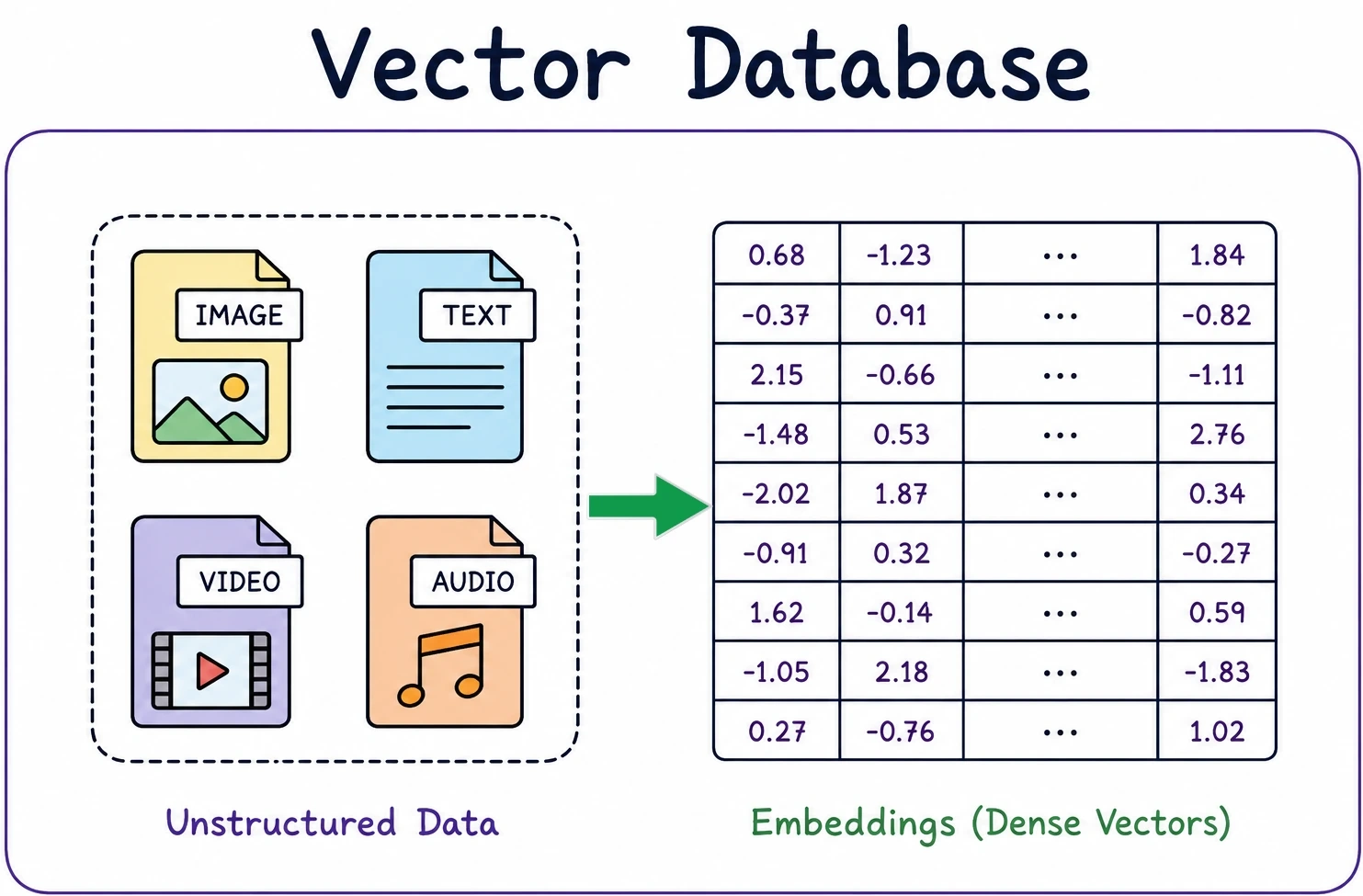
We use a query and find the most similar items in the vector database. When we apply this approach and pass the most similar items to an LLM, then it becomes a RAG (Retrieval Augmented Generation).

But how do we find similarities? we use the embeddings or actual documents and take help of these approaches:

• Distance metrics: L2, cosine, dot product, hamming distance
• Approximate Nearest Neighbor (ANN): IVF, HNSW, PQ fast even at billions of rows, trading a small amount of recall for large speedups
• Metadata filtering: Combining other approaches with filtering

LanceDB and Its Features

LanceDB is an open-source, vector database. It can be used locally, or you can use the enterprise version, or self-host and use LanceDB.

Key features:

1. Multimodal by design: text, vectors, images, audio, and video live as columns in the same table, not as separate data. But you can opt for a mulit-table approach if that works better for you.
2. Multiple index types: IVF / HNSW / PQ / RQ for vectors, BM25 for full text
3. Hybrid search: combine vector similarity and keyword (BM25) search and re-rankers can be used to rank the retrieved documents.
4. Versioning: every write creates a new version; you can checkout, restore, or tag any past version, like Git for your table.
5. Schema changes: add, rename, retype, or drop columns without rewriting the whole dataset, thanks to Lance’s columnar storage.
6. Object storage: the same API works against a local folder or an S3, GS or AZ path.
7. SDKs: Python, TypeScript/JavaScript, and Rust.

Demo

In this section, let’s look at Python examples to use LanceDB to store embeddings, search for similar items, to chunk and index a document, and look at how to store images in the vector tables.

Pre-requisites

You will need an OpenAI key to create the embeddings, you can choose to use any alternatives as well.

Installations

uv pip install lancedb pandas pyarrow pypdf pillow numpy openai open-clip-torch torch

Note: uv is recommended for faster installation

Imports

import io
from getpass import getpass
from pathlib import Path

import lancedb
import numpy as np
import pandas as pd
from pypdf import PdfReader

OPENAI_API_KEY = getpass("Enter your OpenAI API key: ")

Note: Enter the OpenAI key when prompted (If you are using OpenAI’s embedding models)

Initialization

# Local, embedded LanceDB
db = lancedb.connect("./lancedb_data")
print("Connected to local LanceDB at ./lancedb_data")
print("Existing tables:", db.table_names())

Intializing the database locally

Basic vector search example

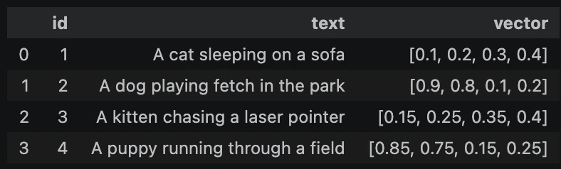
data = [
    {
        "id": 1,
        "text": "A cat sleeping on a sofa",
        "vector": [0.1, 0.2, 0.3, 0.4],
    },
    {
        "id": 2,
        "text": "A dog playing fetch in the park",
        "vector": [0.9, 0.8, 0.1, 0.2],
    },
    {
        "id": 3,
        "text": "A kitten chasing a laser pointer",
        "vector": [0.15, 0.25, 0.35, 0.4],
    },
    {
        "id": 4,
        "text": "A puppy running through a field",
        "vector": [0.85, 0.75, 0.15, 0.25],
    },
]

table = db.create_table("pets", data=data, mode="overwrite")

table.to_pandas()

Note: The numerical vectors here are just example embeddings used to understand vector databases here.

# Query vector close to the "cat" entries
query_vector = [0.12, 0.22, 0.32, 0.4]

results = (
    table.search(query_vector)
    .limit(2)
    .select(["id", "text", "_distance"])
    .to_pandas()
)

results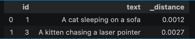

The query is first converted to a vector and then the distance from all the other vectors is calculated, more the distance the less similar the query and text are.

Filtering the table

# Indexed search combined with a metadata filter
filtered_results = (
    table.search(query_vector)
    .where("id != 2")
    .limit(2)
    .select(["id", "text", "_distance"])
    .to_pandas()
)

filtered_results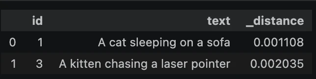

Filtering can be perfomed to exclude or select categories or IDs. You can see the “where” condition in the code.

Creating Vector Index

table.create_index(
    metric="cosine",
    vector_column_name="vector",
    index_type="IVF_FLAT",
)

This syntax can be used to create a vector index of type IVF (inverted file index) and cosine similarity to group similar items together. You can change these parameters according to your needs.

PDF ingestion and retrieval

from pathlib import Path

pdf_path = Path("assets/exploring-ann-algorithms.pdf")

assert pdf_path.exists(), f"Expected a PDF at {pdf_path}"

print(
    f"Using {pdf_path} ({pdf_path.stat().st_size} bytes)"
)

You can use any PDF, or you can download articles (PDF) from Analytics Vidhya for ingestion.

reader = PdfReader(str(pdf_path))

chunks = []

for page_num, page in enumerate(reader.pages):
    text = (page.extract_text() or "").strip()

    if text:
        chunks.append({
            "page": page_num,
            "text": text,
        })

print(f"Extracted text from {len(chunks)} pages")

Extracted text from 14 pages

from openai import OpenAI


def embed_text(text: str) -> list[float]:
    client = OpenAI(api_key=OPENAI_API_KEY)
    response = client.embeddings.create(
        model="text-embedding-3-small",
        input=text,
    )
    return response.data[0].embedding


pdf_rows = [
    {
        "id": f"ann-pdf-p{chunk['page']}",
        "source": pdf_path.name,
        "page": chunk["page"],
        "text": chunk["text"],
        "vector": embed_text(chunk["text"]),
    }
    for chunk in chunks
]

pdf_table = db.create_table(
    "ann_pdf_pages",
    data=pdf_rows,
    mode="overwrite",
)

pdf_table.to_pandas()[["id", "page", "source"]]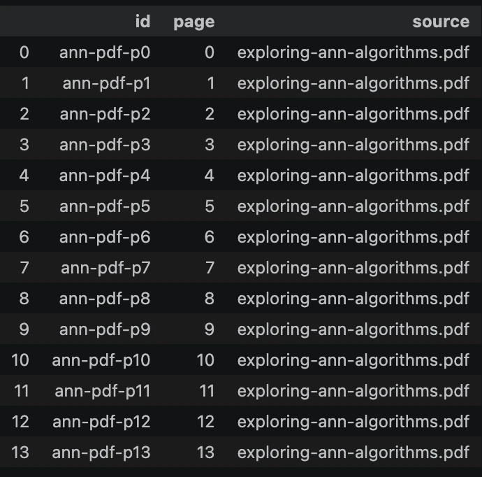

Let’s use an actual embedding model to create the embeddings (text-embedding-3-small from OpenAI). We have chunked the PDF into 14 parts (each page is a chunk) and then embedded them into the vector table.

Example Query

# Semantic search over the PDF's pages
query = "How does the HNSW algorithm find nearest neighbors?"
query_vec = embed_text(query)

matches = (
    pdf_table.search(query_vec)
    .limit(3)
    .select(["id", "page", "text", "_distance"])
    .to_pandas()
)

matches

print(matches["text"][0])

Output:

How HNSW Works 1. As shown in the above image, each vertex in the graph represents a data point. 2. Connect each vertex with a configurable number of nearest vertices in a greedy manner.

Note: You can change the chunking strategy, do it on chunk size (number of chunks) instead of splitting it into varied sized chunks.

Multimodal embedding

from pathlib import Path
from PIL import Image

image_files = {
    "cat": "assets/cat.jpg",
    "dog": "assets/dog.jpg",
    "horse": "assets/horse.jpg",
    "peacock": "assets/peacock.jpg",
}

images_bytes = {}

for label, path in image_files.items():
    p = Path(path)
    assert p.exists(), f"Expected an image at {p}"
    images_bytes[label] = p.read_bytes()
    print(f"Loaded {label}: {path} ({len(images_bytes[label])} bytes)")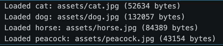

from lancedb.embeddings import get_registry
from lancedb.pydantic import LanceModel, Vector

# Registers LanceDB's built-in OpenCLIP embedding function
clip = get_registry().get("open-clip").create()


class ImageDoc(LanceModel):
    id: str
    image_bytes: bytes = clip.SourceField()
    vector: Vector(clip.ndims()) = clip.VectorField()


images_table = db.create_table(
    "images",
    schema=ImageDoc,
    mode="overwrite",
)

# LanceDB computes vector from image_bytes
images_table.add([
    {"id": label, "image_bytes": data}
    for label, data in images_bytes.items()
])

images_table.to_pandas().drop(columns=["image_bytes"])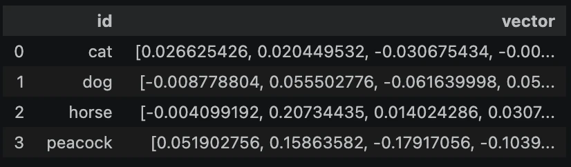

query = "a colorful bird with a fanned tail"

ranked = (
    images_table.search(query)
    .select(["id", "_distance"])
    .to_pandas()
)

print(ranked)

top = ranked.iloc[0]
print(f"\nTop match: {top['id']} (distance={top['_distance']:.4f})")

img = Image.open(io.BytesIO(images_bytes[top["id"]]))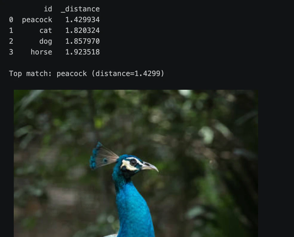

We’re using CLIP via LanceDB to embed the image data into the table. And as you can see it works, the query returns the peacock image as the most similar item.

Potential Applications

Here are some of the use-cases of LanceDB:

• Retrieval-Augmented Generation (RAG): store document chunks and their embeddings, then pass the relevant context into an LLM.
• Semantic and hybrid search: keyword search or keyword search plus meaning-based search together.
• Multimodal search: search images, matching similar audio clips, pulling frames from video, all alongside structured metadata.
• Training and feature stores: Supports datasets for training and evaluation, with schema evolution when you need to add derived features later.
• Anomaly detection: spot duplicate (or almost duplicate) records or outliers using distance-based search.

Conclusion

LanceDB serves well as vector database and more. It combines vectors, metadata, and media in a single versioned, embedded table, with ANN indexing, hybrid search, and object storage support built in. That cuts out a lot of work while building a RAG and search apps. The examples here are just a starting point; things get interesting once you experiment and explore things your own way.

Frequently Asked Questions