Performing Sentiment Analysis Using Twitter Data!

This article was published as a part of the Data Science Blogathon

Photo by Daddy Mohlala on Unsplash

Data is water, purifying to make it edible is a role of Data Analyst – Kashish Rastogi

We are going to clean the twitter text data and visualize data in this blog.

Table Of Contents:

• Problem Statement
• Data Description
• Cleaning text with NLP
• Finding if the text has: with spacy
  • Numbers
  • URL Link
• Cleaning text with preprocessor library
• Analysis of the sentiment of data
• Data visualizing

I am taking the twitter data which is available here on the Analytics Vidhya platform.

Importing libraries

import pandas as pd
import re
import plotly.express as px
import nltk
import spacy

I am loading a small spacy model. There are 3 models size in which you can download spacy (Small, Medium & Large) based on your requirements.

nlp = spacy.load('en_core_web_sm')

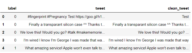
The data looks like this

df = pd.read_csv(r'location of file')
del df['id']
df.head(5)

Problem Statement

Key point is to find the sentiment of the text data. The given text is from customers from various tech firms who manufacture Phones, laptops, Gadgets, etc. The task is to identify if the tweets have a Negative, Positive, or Neutral sentiment towards the company.

Data Description

Label: Label column has 2 unique values 0 & 1.

Tweet: Tweet columns has the text provided by customers

Data Manipulation

Finding the shape of data

There are 2 columns and 7920 rows.

df.shape

Tweets Classification

fig = px.pie(df, names=df.label, hole=0.7, title='Tweets Classification',
             height=250, color_discrete_sequence=px.colors.qualitative.T10)
fig.update_layout(margin=dict(t=100, b=40, l=60, r=40), 
                  plot_bgcolor='#2d3035', paper_bgcolor='#2d3035',
                  title_font=dict(size=25, color='#a5a7ab', family="Lato, sans-serif"),
                  font=dict(color='#8a8d93'),
                  )

Take a moment and look at the data. What do you see?

Image Source: https://unsplash.com/photos/LDcC7aCWVlo

• There is no markup to parse it is plain text (yaa!).
• There are many things to filter out like:

• • The Twitter handle is masked (@user) which of no use for us.
  • Hashtags
  • Links
  • Special characters
• We see the text has numerical value in them.
• There are many typos and contractions in the text.
• There are many company names (Sony, Apple).
• The text is not in lower case

Let’s clean the text

Finding if the text has:

• Twitter user names
• Hashtags
• Numerical values
• Links

Removing if the text has:

• Twitter user name because it won’t provide any additional information right now as for security purposes the username are changed to dummy names
• Hashtag words won’t provide any useful meaning to text in sentiment analysis.
• URL Link won’t add information to text too.
• Removing
  • Punctuation to obtain clean text
  • Word lengths less than 3 are safe to remove from text because words will be like (I’m, are, is) they don’t have any specific meaning and role in the text
  • Stop words is always the best choice to remove

Removing User Name from text

def remove_pattern(input_txt):
    r = re.findall(r"@(w+)", input_txt)
    for i in r:
        input_txt = re.sub(i, '', input_txt)      
    return input_txt
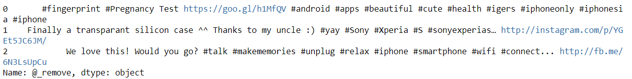
df['@_remove'] = np.vectorize(remove_pattern)(df['tweet'])
df['@_remove'][:3]

Finding Hashtags in text

hashtags = []
def hashtag_extract(x):
    # Loop over the words in the tweet
    for i in x:
        ht = re.findall(r"#(w+)", i)
        hashtags.append(ht)
    return hashtags

 

Passing function & extracting hashtags now we can visualize how many hashtags are there in positive & negative tweets

# extracting hashtags from neg/pos tweets
dff_0 = hashtag_extract(df['tweet'][df['label'] == 0])
dff_1 = hashtag_extract(df['tweet'][df['label'] == 1])
dff_all = hashtag_extract(df['tweet'][df['label']])
# unnesting list
dff_0 = sum(dff_0,[])
dff_1 = sum(dff_1,[])
dff_all = sum(dff_all,[])

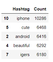
Counting frequent hashtags used when label=0. FreqDist means it will tell us how many times that word came in the whole document.

data_0 = nltk.FreqDist(dff_0)
data_0 = pd.DataFrame({'Hashtag': list(data_0.keys()),
                  'Count': list(data_0.values())}).sort_values(by='Count', ascending=False)
data_0[:5]

 

If you want to know more about Plotly and how to use it do visit this blog. Every graph is well explained with different parameters that you need to take care of while plotting charts.

fig = px.bar(data_0[:30], x='Hashtag', y='Count', height=250,
             title='Top 30 hashtags',
             color_discrete_sequence=px.colors.qualitative.T10)
fig.update_yaxes(showgrid=False),
fig.update_xaxes(categoryorder='total descending')
fig.update_traces(hovertemplate=None)
fig.update_layout(margin=dict(t=100, b=0, l=60, r=40), 
                  hovermode="x unified",
                  xaxis_tickangle=300,
                  xaxis_title=' ', yaxis_title=" ",
                  plot_bgcolor='#2d3035', paper_bgcolor='#2d3035',
                  title_font=dict(size=25, color='#a5a7ab', family="Lato, sans-serif"),
                  font=dict(color='#8a8d93')
                  )

Passing text

sentences = nlp(str(text))

Finding Numerical Values in text

spacy provides functions like_num which tells if the text has numerical values in them or not

for token in sentences:
    if token.like_num:
        text_num = token.text
print(text_num)

Finding URL Link in the text

spacy provides function like_url which tells if the text has a URL Link in them or not

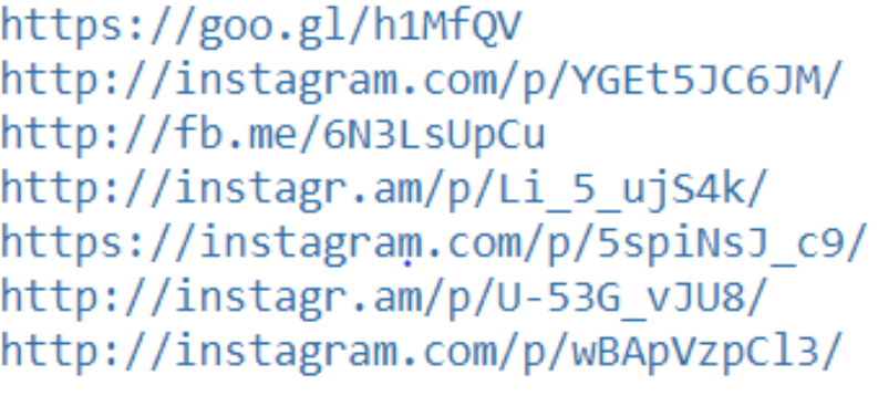
# find links
for token in sentences:
    if token.like_url:
        text_links = token.text
        print(text_links)

There is a library in python which helps to clean text you can find the documentation here

Currently, this library supports cleaning, tokenizing, and parsing

• URLs
• Hashtags
• Mentions
• Reserved words (RT, FAV)
• Emojis
• Smileys

Importing library

!pip install tweet-preprocessor
import preprocessor as p

Calling a function to clean the text

def preprocess_tweet(row):
    text = row['tweet']
    text = p.clean(text)
    return text

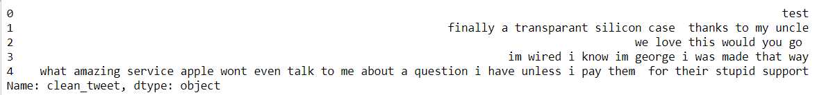
df['clean_tweet'] = df.apply(preprocess_tweet, axis=1)
df[:6]

 

As we see clean_tweet columns has only text all the usernames, hashtag and URL Links are removed

Some of the steps for cleaning are remaining like

• lowering all the text
• Removing punctuations
• Removing numbers

Code:

def preprocessing_text(text):
     # Make lowercase
     text = text.str.lower()
     # Remove punctuation
     text = text.str.replace('[^ws]', '', regex=True)
     # Remove digits
     text = text.str.replace('[d]+', '', regex=True)
     return text
 pd.set_option('max_colwidth', 500)
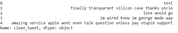
 df['clean_tweet'] = preprocessing_text(df['clean_tweet'])
 df['clean_tweet'][:5]

 

We got our clean text let’s remove stop words.

What are Stop words? Is it necessary to remove stop words?

Stopwords are the most common words in any natural language. Stop words are like I, are, you, When, etc they don’t add any additional information to text.

It is not necessary to remove stop words every time it depends on the case study, here we are finding the sentiment of the text so we don’t need to stop words.

from nltk.corpus import stopwords
# Remove stop words
stop = stopwords.words('english')
df['clean_tweet'] = df['clean_tweet'].apply(lambda x: ' '.join([word for word in x.split() if word not in (stop)]))
df['clean_tweet'][:5]

After implementing all the steps we got our clean text. Now what to do with text?

• We can find out which words are frequently used?
• Which words are negatively/positively used more in the text?

Tokenizing words and calculating the frequency and word count & storing them in a data frame.

A frequency distribution records the number of times each word has occurred. For example, a new word has been used frequently in whole data followed by other words iPhone, phone, etc.

a = df['clean_tweet'].str.cat(sep=' ')
words = nltk.tokenize.word_tokenize(a)
word_dist = nltk.FreqDist(words)
dff = pd.DataFrame(word_dist.most_common(), 
                    columns=['Word', 'Frequency'])
dff['Word_Count'] = dff.Word.apply(len)
dff[:5]

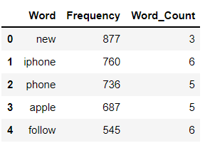
fig = px.histogram(dff[:20], x='Word', y='Frequency', height=300, 
                   title='Most common 20 words in tweets', color_discrete_sequence=px.colors.qualitative.T10)
fig.update_yaxes(showgrid=False),
fig.update_xaxes(categoryorder='total descending')
fig.update_traces(hovertemplate=None)
fig.update_layout(margin=dict(t=100, b=0, l=70, r=40),
                        hovermode="x unified",
                        xaxis_tickangle=360,
                        xaxis_title=' ', yaxis_title=" ",
                        plot_bgcolor='#2d3035', paper_bgcolor='#2d3035',
                        title_font=dict(size=25, color='#a5a7ab', family="Lato, sans-serif"),
                        font=dict(color='#8a8d93'),
                          )

fig = px.bar(dff.tail(10), x='Word', y='Frequency', height=300, 
                   title='Least common 10 words in tweets', color_discrete_sequence=px.colors.qualitative.T10)
fig.update_yaxes(showgrid=False),
fig.update_xaxes(categoryorder='total descending')
fig.update_traces(hovertemplate=None)
fig.update_layout(margin=dict(t=100, b=0, l=70, r=40),
                        hovermode="x unified",
                        xaxis_title=' ', yaxis_title=" ",
                        plot_bgcolor='#2d3035', paper_bgcolor='#2d3035',
                        title_font=dict(size=25, color='#a5a7ab', family="Lato, sans-serif"),
                        font=dict(color='#8a8d93'),
                          )

fig = px.bar(a, height=300, title='Frequency of words in tweets', 
             color_discrete_sequence=px.colors.qualitative.T10)
fig.update_yaxes(showgrid=False),
fig.update_xaxes(categoryorder='total descending')
fig.update_traces(hovertemplate=None)
fig.update_layout(margin=dict(t=100, b=0, l=70, r=40), showlegend=False,
                        hovermode="x unified",
                        xaxis_tickangle=360,
                        xaxis_title=' ', yaxis_title=" ",
                        plot_bgcolor='#2d3035', paper_bgcolor='#2d3035',
                        title_font=dict(size=25, color='#a5a7ab', family="Lato, sans-serif"),
                        font=dict(color='#8a8d93'),
                          )

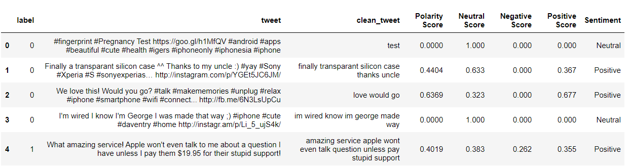
Sentiment Analysis

from nltk.sentiment.vader import SentimentIntensityAnalyzer
from nltk.sentiment.util import *
#Sentiment Analysis
SIA = SentimentIntensityAnalyzer()
df["clean_tweet"]= df["clean_tweet"].astype(str)
# Applying Model, Variable Creation
df['Polarity Score']=df["clean_tweet"].apply(lambda x:SIA.polarity_scores(x)['compound'])
df['Neutral Score']=df["clean_tweet"].apply(lambda x:SIA.polarity_scores(x)['neu'])
df['Negative Score']=df["clean_tweet"].apply(lambda x:SIA.polarity_scores(x)['neg'])
df['Positive Score']=df["clean_tweet"].apply(lambda x:SIA.polarity_scores(x)['pos'])
# Converting 0 to 1 Decimal Score to a Categorical Variable
df['Sentiment']=''
df.loc[df['Polarity Score']>0,'Sentiment']='Positive'
df.loc[df['Polarity Score']==0,'Sentiment']='Neutral'
df.loc[df['Polarity Score']<0,'Sentiment']='Negative'
df[:5]

Tweets Classification based on sentiment

fig_pie = px.pie(df, names='Sentiment', title='Tweets Classifictaion', height=250,
                 hole=0.7, color_discrete_sequence=px.colors.qualitative.T10)
fig_pie.update_traces(textfont=dict(color='#fff'))
fig_pie.update_layout(margin=dict(t=80, b=30, l=70, r=40),
                      plot_bgcolor='#2d3035', paper_bgcolor='#2d3035',
                      title_font=dict(size=25, color='#a5a7ab', family="Lato, sans-serif"),
                      font=dict(color='#8a8d93'),
                      legend=dict(orientation="h", yanchor="bottom", y=1, xanchor="right", x=0.8)
                      )

Conclusion:

We saw how to clean text data when we have a Twitter username, hashtag, URL Links, digits and did sentiment analysis on text data.

We saw how to find if the text has URL links or digits in them with the help of spacy.

About the author:

You can connect me

Linkedin

Medium

The media shown in this article are not owned by Analytics Vidhya and are used at the Author’s discretion.

Kashish Rastogi 15 Jul 2021

A student who is learning and sharing with a storyteller to make your life easy.