How to Use KV Caching in LLMs?

LLMs have been a trending topic lately, but it’s always interesting to understand how these LLMs work behind the scenes. For those unaware, LLMs have been in development since 2017’s release of the famed research paper “Attention is all you need”. But these early transformer-based models had quite a few drawbacks due to heavy computation and memory requirements from the internal math.

As we generate more and more text in our LLMs, we start to consume more GPU memory. At a certain point, our GPU gets an Out of Memory issue, causing the complete program to crash, leaving the LLM unable to generate any more text. Key-Value caching is a technique that helps mitigate this. It basically remembers important information from previous steps. Instead of recomputing everything from scratch, the model reuses what it has already calculated, making text generation much faster and more efficient. This technique has been adopted in several models, like Mistral, Llama 2, and Llama 3 models.

So let’s understand why KV Caching is so important for LLMs.

TL;DR

• KV Caching stores previously computed Keys/Values, so transformers skip redundant work.
• It massively reduces computation but becomes memory-bound at long sequence lengths.
• Fragmentation & continuous memory requirements lead to low GPU utilization.
• Paged Attention (vLLM) fixes this using OS-style paging + non-contiguous memory blocks.

The Attention Mechanism

We normally generate 3 different weight matrices (W_q, W_k, W_v) to produce our Q, K, and V vectors. These weight matrices are derived from the data.

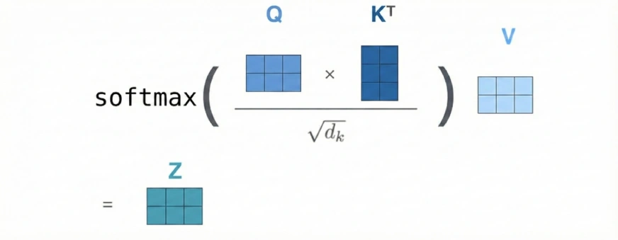
We can consider our Q to be a vector and the K and V to be 2D matrices. This is because K and V store one vector per previous token, and when stacked together, form matrices.

The Q vector represents the new token that comes in the decoder step.

Meanwhile, the K matrix represents the information or “keys” of all previous tokens that the new token can query to decide relevance.

Whenever a new Query vector is input, it compares itself with all the Key vectors. It basically figures out which previous tokens matter the most.

This relevance is represented through the weighted average known as the soft attention score.

The V matrix represents the content/meaning of each previous token. Once the attention scores are computed, they are used to take a weighted sum of the V vectors. They produce the final contextual output that the model uses for the next steps.

In simple terms, K helps decide what to look at, and V provides what to take from it.

What was the issue?

In a typical causal transformer, which does autoregressive decoding, we generate one word at a time, provided we have all the previous context. As we keep generating one token at a time, the K and V matrices get appended to newer values. Once the embedding is computed for this value, the corresponding value won’t change at all. But the model has to do some heavy computations for the K and V matrices for this corresponding value on all the steps. This results in a quadratic number of matrix multiplications. A very heavy and slow task.

Why we need KV Caching

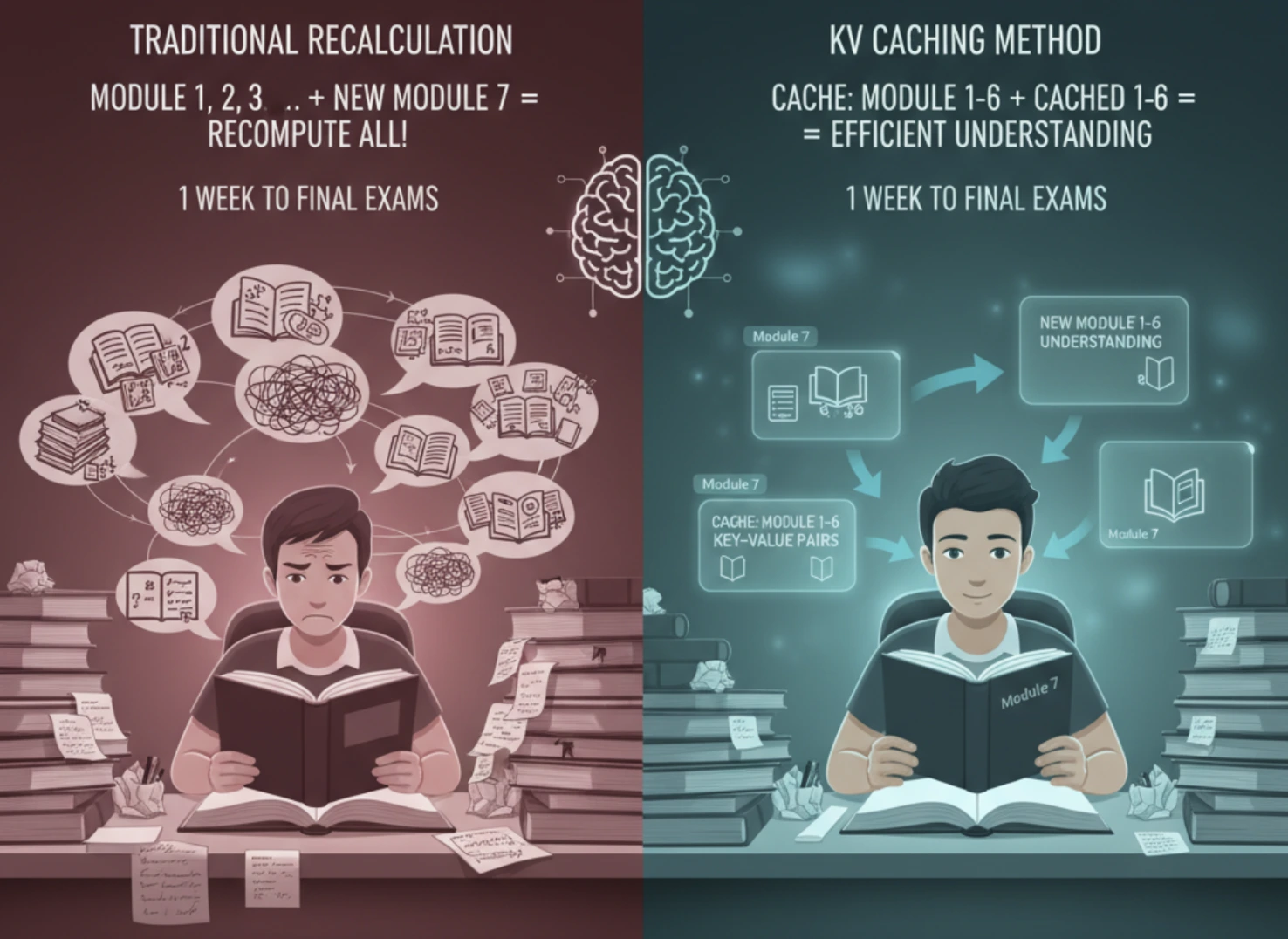
Let’s try to understand this with a real-life example – An Exam Preparation Scenario

We have our final exams in a week and 20 modules to study in 7 days. We start with the first module, which can be thought of as the first token. After finishing it, we move on to the second module and naturally try to relate it to what we learned earlier. This new module (the second token), interacting with the previous modules, is similar to how a new token interacts with earlier tokens in a sequence.

This relationship is important for understanding. As we continue studying more modules, we still remember the content of the previous ones, and our memory acts like a cache. So, when learning a new module, we only think about how it connects to earlier modules instead of re-studying everything from the beginning each time.

This captures the core idea of KV Caching. The K and V pairs are stored in memory from the start, and whenever a new token arrives, we only compute its interaction with the stored context.

How KV Caching helps

As you can see, KV Caching saves a huge amount of computation because all previous K and V pairs are stored in memory. So when a new token arrives, the model only needs to compute how this new token interacts with the already-stored tokens. This eliminates the need to recompute everything from scratch.

With this, the model shifts from being compute-bound to memory-bound, making VRAM the main limitation. In regular multi-head self-attention, every new token requires full tensor operations where Q, K, and V are multiplied with the input, leading to quadratic complexity. But with KV Caching, we only do a single row (vector-matrix) multiplication against the stored K and V matrices to get attention scores. This drastically reduces compute and makes the process more limited by memory bandwidth than raw GPU compute.

KV Caching

The core idea behind KV Caching is simple: Can we avoid recomputing work for tokens the model has already processed during inference?

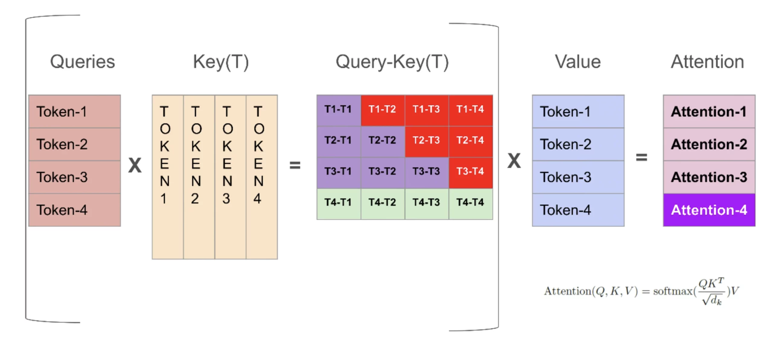
In the above image, we see the reddish area to be redundant since we only care about the computation of the next row in Q-K(T).

Here, K corresponds to the Key Matrix and V corresponds to the Value Matrix.

When we calculate the next token in a causal transformer, we only need the most recent token to predict the following one. This is the basis of next-word prediction. Since we only query the nth token to generate the n+1th token, we do not need the old Q values and therefore do not store them. But in standard multi-head attention, Q, K, and V for all tokens are recomputed repeatedly because we do not cache the keys and values.

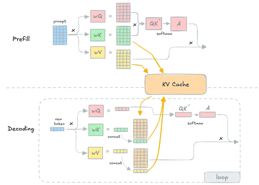
In the above image, K and V represent the accumulated context from all the previous tokens. Before KV Caching existed, the model would recompute all the K and V matrices from the beginning up to the latest token at every decoding step. This also meant recomputing all soft attention scores and final attention outputs repeatedly, which is compute-intensive. With KV Caching, however, we store all K vectors up to sequence length − 1, and do the same for the V matrix from 1 to n−1.

Since we only need to query the latest token, we don’t recompute the older tokens anymore. The nth token already contains all the information required to generate the (n+1)th token.

KV Caching: The Core Idea

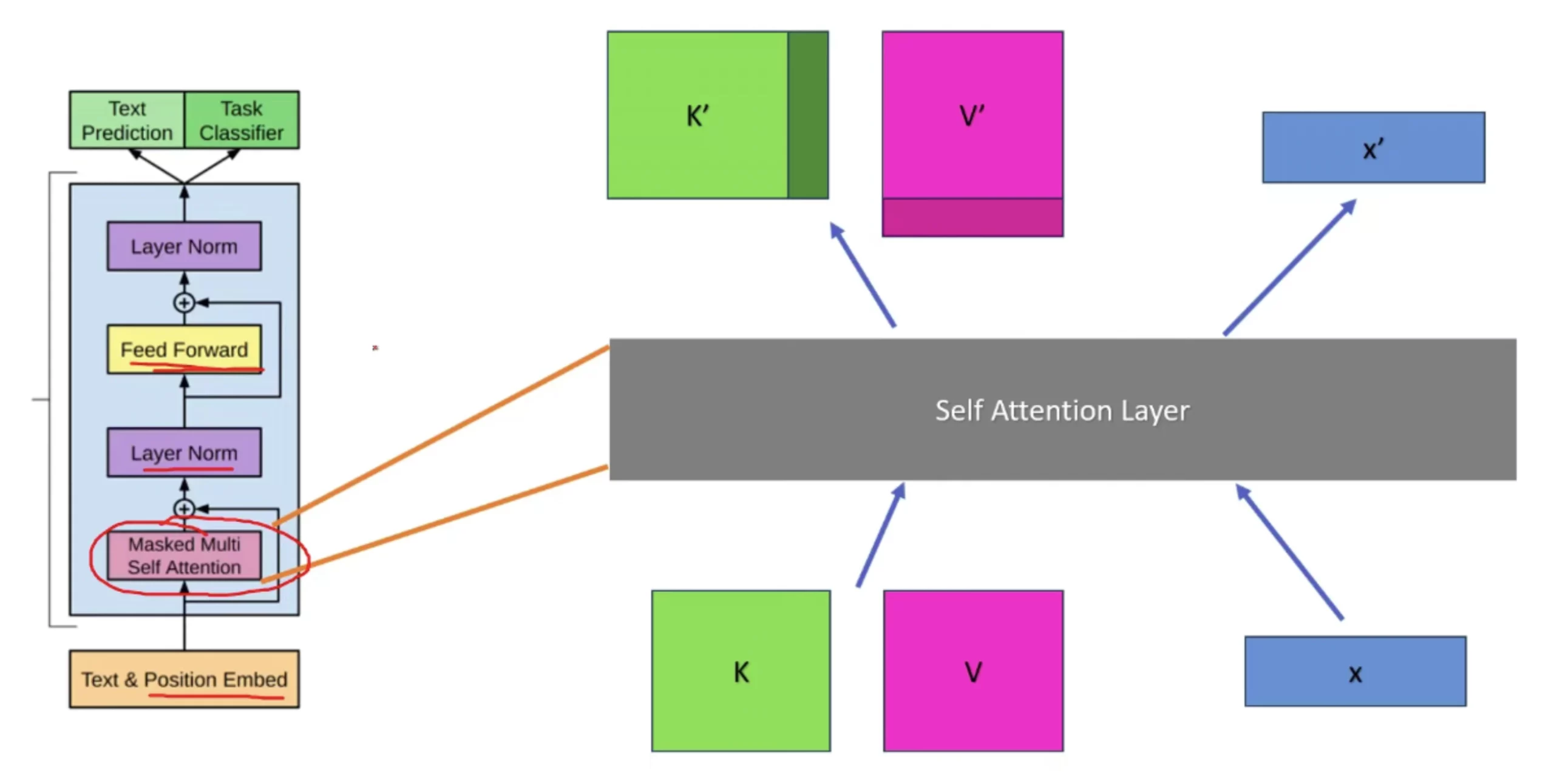
The main idea of KV Caching starts from here…

Whenever a new token arrives, we compute its new K vector and append it as an additional column to the existing K matrix, forming K’. Similarly, we compute the new V vector for the latest token and append it as a new row to form V’. This is a lightweight tensor operation.

Illustration

If this feels confusing, let’s break it down with a simple illustration.

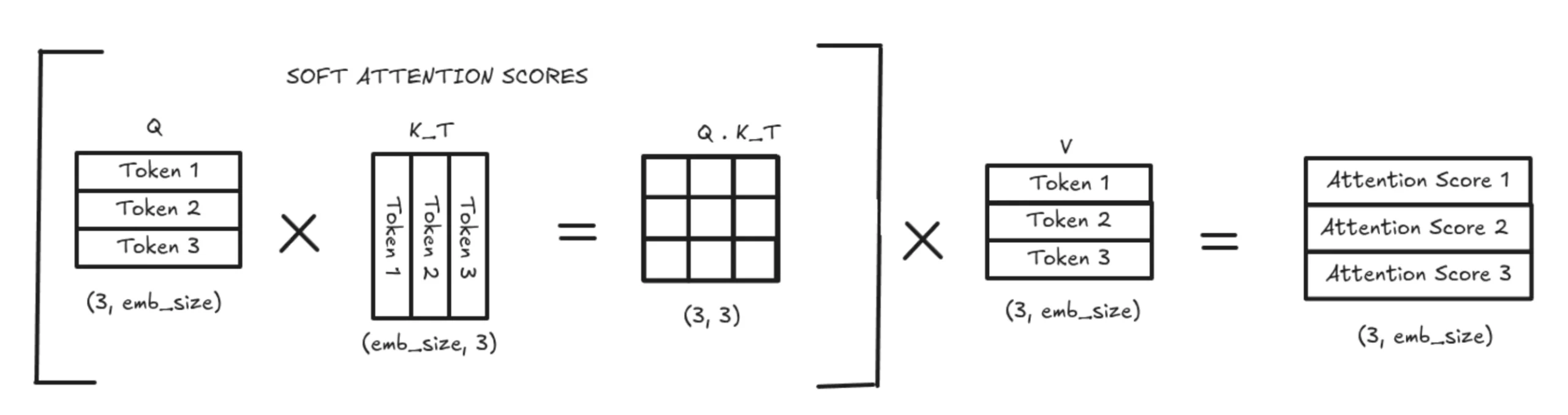
Without KV Caching, the model recomputes the entire K and V matrices every time. This results in a full quadratic-size attention computation to produce soft attention scores, which are then multiplied by the entire V matrix. This is extremely expensive in both memory and computation.

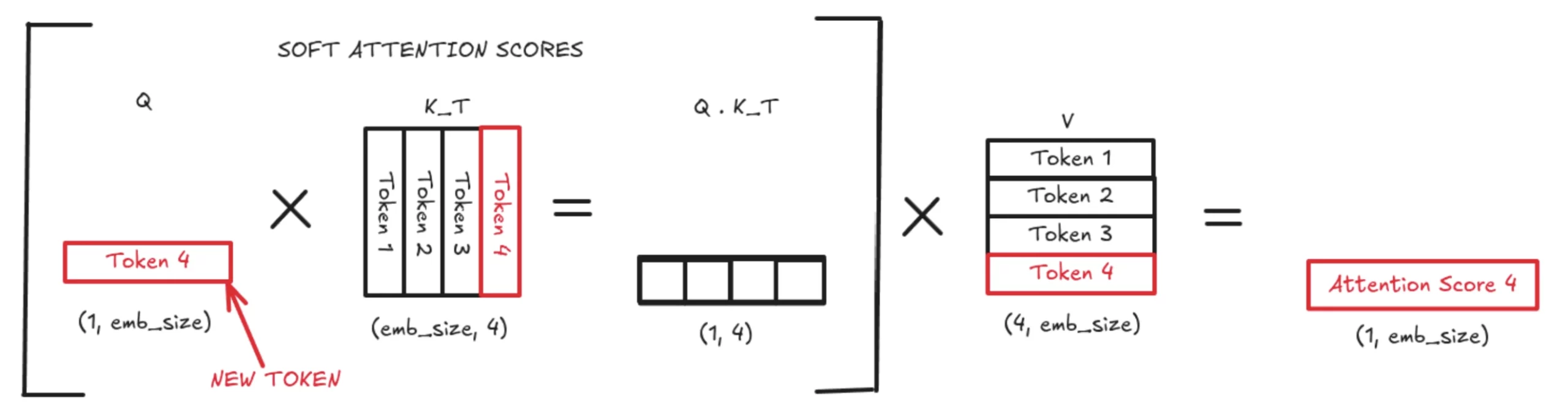
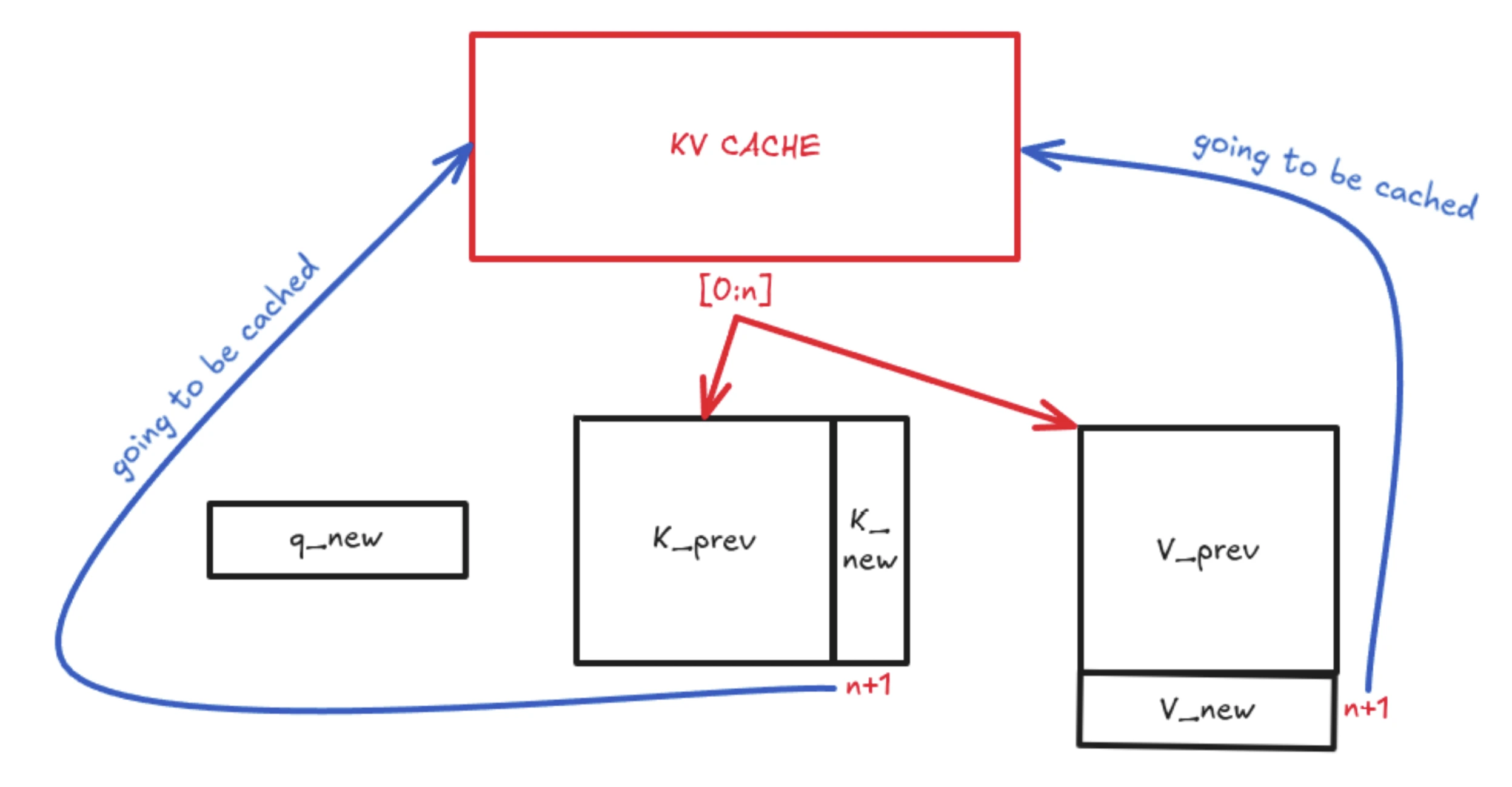
With KV Caching, we only use the latest token’s query vector (q_new). This q_new is multiplied by the updated K matrix, which contains both K_prev (cached) and K_new (just computed). The same logic applies to V_prev, which gets a new V_new row. This greatly reduces computation by turning a large matrix-matrix multiplication into a much smaller vector-matrix multiplication. The resulting attention score is appended to the attention matrix and used normally in the transformer flow.

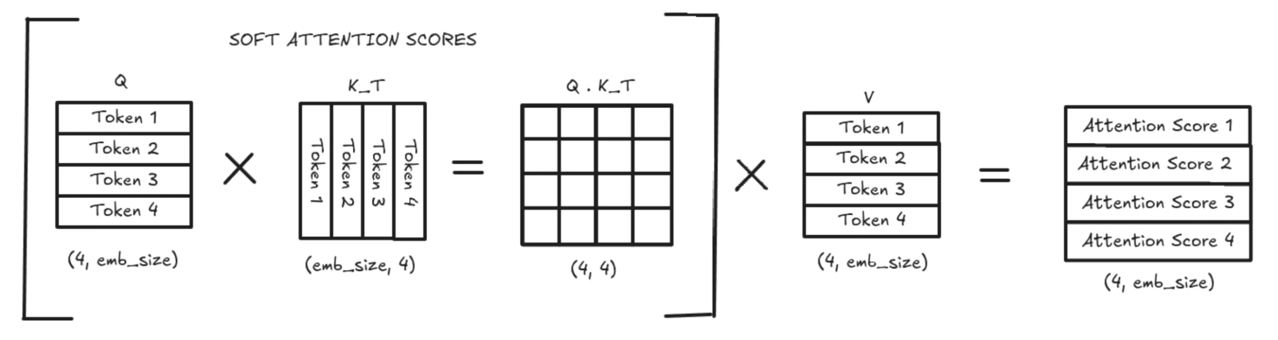
This 4th attention value (in this example) is then used to compute the next token. With KV Caching, we do not store or recompute previous Q values, but we do store all previous K vectors. The new Q is multiplied by Kᵀ to get the Q·Kᵀ vector (the soft attention scores). These scores are multiplied by the V matrix to produce a weighted average over the stored context, which becomes the 4th token’s output used for prediction.

Attention only depends on preceding tokens. This operation depends on GPU’s VRAM, so we need to store these K and V matrices. So, effectively, that’s the upper limit for us as a memory constraint.

There are also several mentions of KV heads in research papers like Llama 2, because we know transformers have several layers, and each layer has several heads. For each head KV cache is applied on it, hence the name KV head.

Challenges of KV Cache

The challenges we face in KV Caching are:-

• Low GPU Utilization: Despite having powerful GPUs, KV caching often uses only 20-40% of GPU VRAM, mainly due to memory being allocated in ways that cannot be fully used.
• Continuous Memory Requirement: KV cache blocks must be stored in contiguous memory, making allocation stricter and leaving many small free gaps unusable.

When dealing with KV Cache, GPU memory doesn’t get used perfectly even though GPUs are excellent at handling fast, iterative operations. The problem lies in how memory is carved up and reserved for token generation.

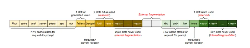
Internal Fragmentation

Internal fragmentation happens when you allocate more memory than you actually use. For example, if a model supports a max sequence length of 4096 tokens, we must pre-allocate space for all 4096 positions. But in reality, most generations might end at 200-500 tokens. So, even though memory for 4096 tokens is sitting there reserved and ready, only a small chunk is actually filled. The remaining slots stay empty. This wasted space is internal fragmentation.

External Fragmentation

External fragmentation occurs when memory is available but not in one clean, continuous block. Different requests start and finish at different times. This leaves tiny “holes” in memory that are too small to be reused efficiently. Even though the GPU has VRAM left, it can’t fit new KV cache blocks because the free memory isn’t contiguous. This leads to low memory utilization even though, technically, memory exists.

Reservation Issue

The reservation problem is basically pre-planning gone wrong. We reserve memory as if the model will always generate the longest possible sequence. But generation might stop much earlier (EOS token, or hitting an early stopping criteria). This means large chunks of reserved KV cache memory never get touched yet remain unavailable for other requests.

Paged Attention

Paged Attention (used in vLLM) fixes the fragmentation problem by borrowing ideas from how operating systems manage memory. Just like an OS does paging, vLLM breaks the KV cache into small, fixed-size blocks instead of reserving one large continuous chunk.

• Logical Blocks: Each request sees a clean, continuous sequence of KV memory logically. It thinks its tokens are stored one after another, just like normal attention.
• Physical Blocks: Under the hood, these “logical blocks” are actually scattered across many non-contiguous physical memory pages in GPU VRAM. vLLM uses a Block Table (just like a page table in OS) to map logical positions -> physical locations.

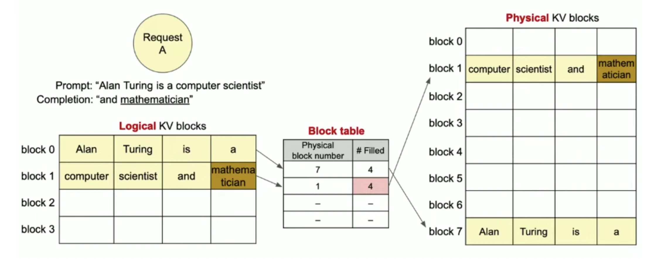
So instead of needing one large 4096 slot continuous buffer, Paged Attention stores tokens in small blocks (like pages) and arranges them flexibly in memory.

This means:

• No more internal fragmentation
• No need for continuous VRAM
• Instant reuse of free blocks
• GPU utilization jumps from ~20-40% to ~96%

But we won’t be covering this concept in depth here. Maybe in the upcoming blogs.

Memory Consumption of KV Cache

To understand how much memory KV cache consumes for a certain model, we need to understand the following 4 variables here:-

• num_layers (number of layers in the transformer model)
• num_heads (KV head for each head in the multi-head self-attention layer)
• head_dim (the dimension of each KV head)
• precision_in_bytes (let’s take 16 bits which is 2 bytes)(FP16 => 16 bits = 2 bytes)

Let’s assume the following values for our use case: num_layers = 32, num_heads = 32, head_dim = 128, and batch_size = 1 (actual deployments usually have higher batches).

Let’s now calculate KV cache per token.

KV cache per token = 2 * (num_layers) * (num_heads * head_dim) * precision_in_bytes * batch_size

Why the 2?

Because we store two matrices per token – K and V matrices

KV cache per token = 2 * 32 * (32 * 128) * 2 * 1
= 524288 B
= 0.5 MB

We need 0.5 MB to store KV per token across all the layers and heads. Shocker!!!

Consider the Llama 2 model, we know we have 4096 sequence length if we want to do 1 request. If we are requesting earlier than for every request, if we are using KV cache, we need to store all of this information.

Total KV cache per request = seq_len * KV cache per token
= 4096 * 524288
= 2147483648 / (1024 * 1024 * 1024)
= 2 GB

So basically, we need 2 GB per request. KV cache is needed for 1 request.

Conclusion

In this blog, we discussed the underlying working of KV Caching and its purpose. In doing so, we learnt why it is such an important optimization for contemporary LLMs. We looked at how transformers initially had trouble with high computation and memory requirements. And how KV caching significantly reduces redundant work by storing previously calculated Key and Value vectors.

Then, we looked into the actual problems with KV caching, such as low GPU utilization. The requirement for contiguous memory, and how problems like reservation, internal fragmentation, and external fragmentation result in significant VRAM waste.

We also briefly discussed how Paged Attention (vLLM) resolves these problems using OS style paging logic. It allows KV cache to grow in small, reusable pieces rather than massive, rigid chunks, significantly increasing GPU memory utilization.

Lastly, we analysed the computation of KV Cache memory consumption. We observed that on a model like Llama-2, a single request can easily use almost 2 GB of VRAM for KV storage. Wild stuff.

If you want me to go into further detail on Paged Attention, block tables, and the reasons for vLLM’s fast throughout… Let me know in the comments below, and I shall attempt to cover the same in my next blog. Until then!