Excel 101: Complete Guide to VLOOKUP Function

Try the following – ask any Excel user for his/ her favourite Excel formula. More often than not, you will hear just this one name -VLOOKUP. And this fame is for all the right reasons. From finance teams reconciling numbers to analysts cleaning messy datasets, this function quietly powers the most crucial operations in a spreadsheet. So, yes, if you do not already, you should know all about VLOOKUP.

And if this importance is clear to you, and you are reading this article to learn VLOOKUP, kudos! You are at the right place, as here, we shall explore all there is to know about VLOOKUP, how it works, and what all you can do with it. The best part – we will go through this learning experience with real examples.

So, follow along, and be a master of VLOOKUP in no time.

What is VLOOKUP?

First things first. What does “VLOOKUP” even mean? The name comes from a simple logic it follows – Vertical Lookup. In essence, it is an Excel function that searches for a value, as indicated by the “lookup” moniker. But it does so in a very specific manner.

It looks for the value in the first column of a table and returns a corresponding value from another column in the same row. The function works vertically (top to bottom), which is where the name comes from.

Think of it as Excel’s way of saying: “Find this item, then bring me the detail associated with it.”

In simple terms, VLOOKUP helps you:

• Match data between two tables
• Retrieve related information instantly
• Eliminate manual searching and copy-pasting
• Reduce errors in repetitive data tasks

Here is a look at its importance in detail.

Also read: Microsoft Excel for Data Analysis

How VLOOKUP Helps

We know now that at its core, VLOOKUP solves one of the most common problems in data work: finding the right value in seconds. As an example, if you have a list of product names and prices, VLOOKUP can quickly find the price of a specific product without you manually scanning the table.

Now simply imagine this list scaled 1000 times.

Because that is the kind of data volume that big corporations work with. Multiple spreadsheets house data points in thousands, and manually sifting through such data is like finding a needle in a haystack.

This is where VLOOKUP shines. No matter the volume of the data, VLOOKUP will work just as fine across gigantic spreadsheets too. In such scenarios, whether you’re matching product prices or IDs, merging reports, or building dashboards, it is easy to see how mastering VLOOKUP can save hours of manual effort.

Here are some real-life use cases where VLOOKUP is used on a daily basis:

• Fetching product prices from a master pricing sheet
• Matching customer IDs with names, emails, or purchase history
• Pulling employee details (department, role, salary band) from HR databases
• Mapping order IDs to order status in operations reports
• Merging sales data from multiple regional spreadsheets into one report
• Retrieving inventory levels for specific SKUs from warehouse records
• Linking invoice numbers to payment status in finance trackers

and the list goes on. Hopefully, this gives youa. gist of just how important VLOOKUP can prove to be. Now that the requirement is clear, let’s move on to actually understanding the function.

Understanding VLOOKUP

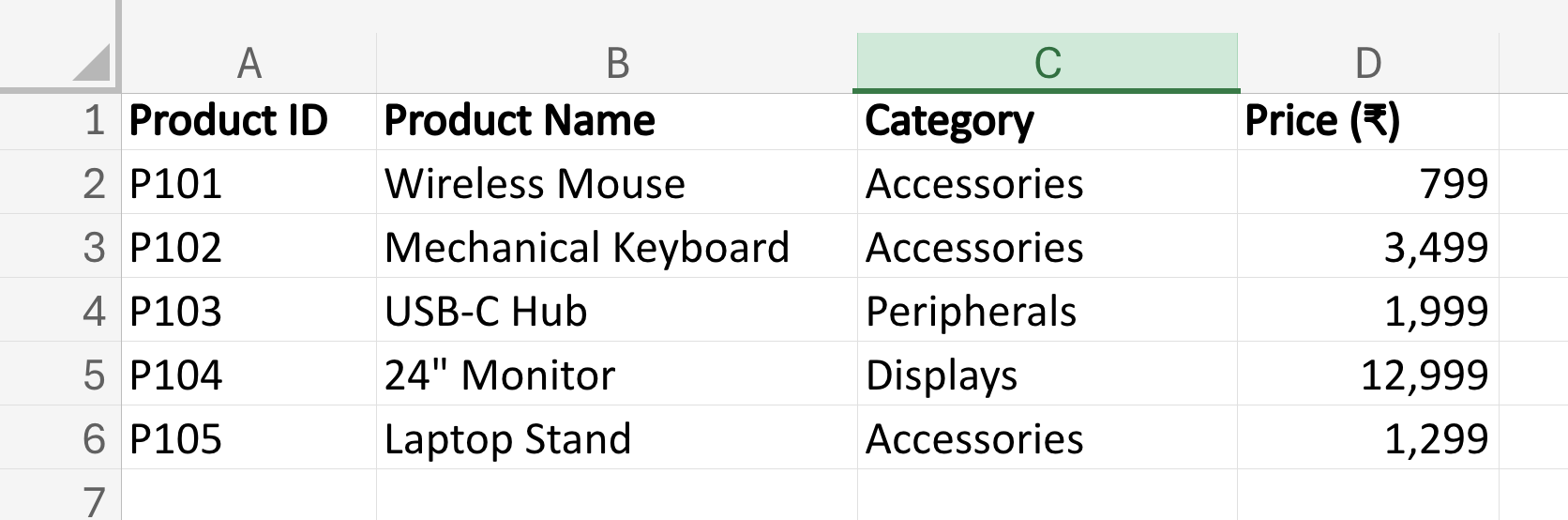
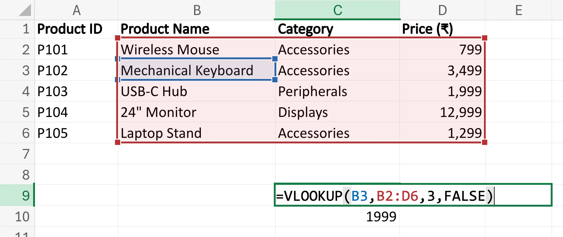
Let us try to understand VLOOKUP with an example. Consider the data in the screenshot below. It lists the products in an IT warehouse, along with their product IDs and associated costs. I have kept this list short for utmost clarity in understanding the function.

Now, imagine you wish to find the price of the Mechanical Keyboard from this list. Here is the VLOOKUP formula for the same:

=VLOOKUP(B3,B2:D6,3,FALSE)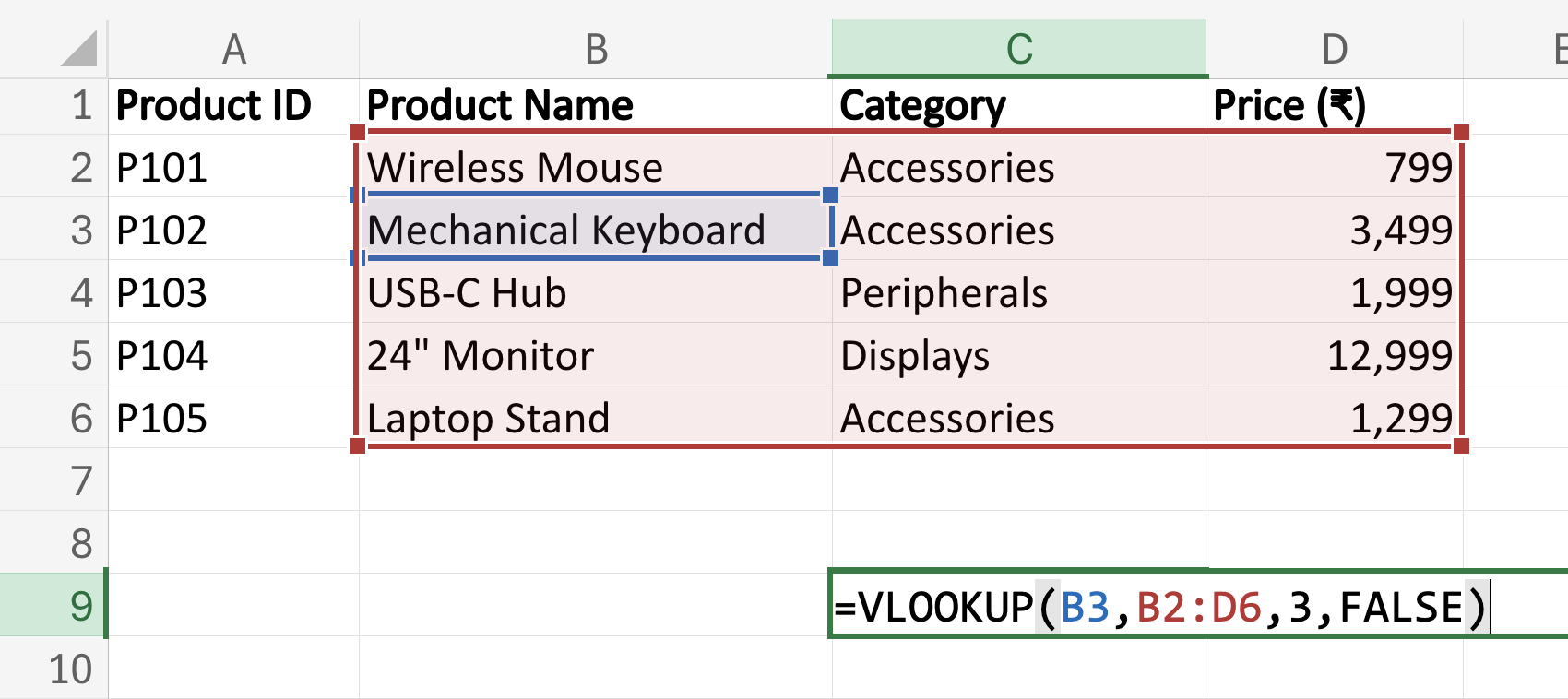

This may seem complex at first, but don’t worry, we will walk through this step by step.

Let us begin with the terminology of the different elements involved here, and the syntax that the formula follows.

VLOOKUP Syntax

To make VLOOKUP work, you only need four inputs – nothing more. These are:

• Lookup value: the value you want to search for. In our example, this is Mechanical Keyboard, since we wish to find its price.
• Table range: where the data lives. In our case, this is complete columns B to D.
  Important: the lookup value must be in the first column of this range.
• Column index number: which column contains the value you want returned. (If your range is B:D, then B=1, C=2, D=3.)
• Match type: This is optional in most cases. Here are the two types:
  FALSE = exact match (most common)
  TRUE = approximate match (default if you leave it blank)

That’s it! These are the four inputs between you and never manually searching a spreadsheet again.

For effectively using VLOOKUP, just put it all together as follows:

=VLOOKUP(lookup_value, table_range, column_index, FALSE/True)

Forming the Formula

Now, let us compare this with the VLOOKUP formula we came up with for our example above.

=VLOOKUP(B3,B2:D6,3,FALSE)

• As you can see in the table, the term “Mechanical Keyboard” is placed at B3, and that is our lookup_value. So we simply specify its position in the first instance.
• Next, we share the table_range, which in our case, is B2 to D6, as all the data is between these columns.
• Next, we specify the column number from which we want the data. Since it is price, it is under the ‘D’ column, which is the third column from our table_range (B=1, C=2, D=3). Hence the 3.
• Lastly, we choose if we want an exact match of the query, or just an approximate match. Since we want an exact match, we will use False.

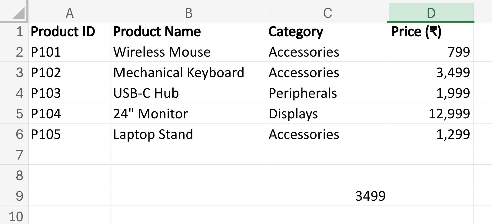
And that’s it! Our VLOOKUP formula is ready to use. As you can see in the table, we have correctly found our answer, i.e. a price of Rs 3,499 for the Mechanical Keyboard.

Just to test if you’ve got it, try framing the VLOOKUP formula for finding the price of Laptop Stand. I’ll mention the correct answer at the end of this article.

Assuming you are clear with the basic concepts of VLOOKUP, let’s explore some special scenarios in which it may require some tweaks.

Also read: Best Resources to learn Microsoft Excel

Absolute References in VLOOKUP

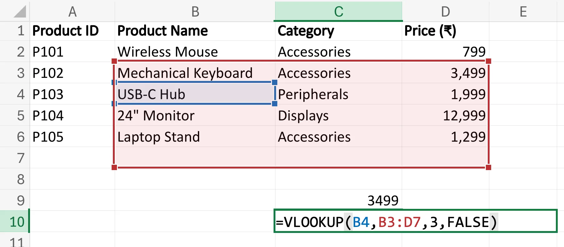
If you try copying your VLOOKUP formula down a column, you will face an unexpected problem: the formula breaks. Instead of returning correct values, you might see errors or incorrect results. This happens because Excel shifts the table range whenever the VLOOKUP formula is copied. This is known as relative referencing.

By default, Excel assumes that references should move with the formula. So if your table range is B2:D6 and you copy the formula down one row, Excel adjusts it to B3:D7. The result? Your lookup table shifts… and your data may disappear.

This is where absolute references save the day.

An absolute reference locks the table range so it does not move when copied. You create it by adding dollar signs. So the regular table_range becomes something like this:

B2:D6 → $B$2:$D$6

You can do this instantly by selecting the range in your formula and pressing F4.

When do you need this?

Imagine you are filling prices for 100 products using one master price table. Instead of writing the formula 100 times, you write it once and drag it down. Without absolute references, the lookup table keeps shifting, and the results break. With $B$2:$D$6, the formula always points to the correct range in the table.

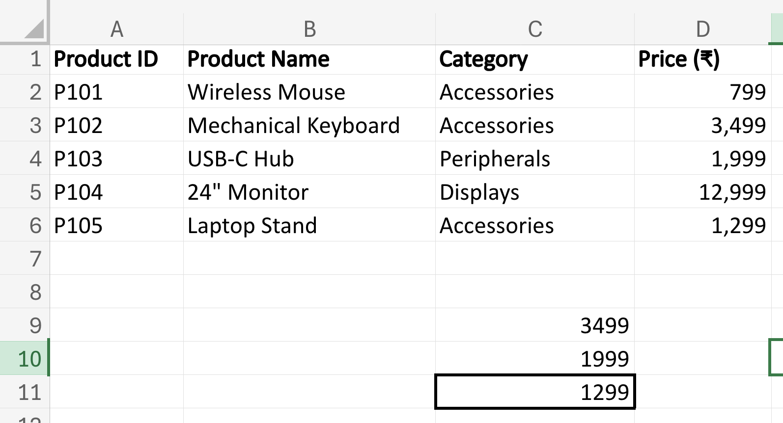
Checkout how the range shifts in the screenshots below, when I copy/paste the VLOOKUP formula just one row below. B2:D6 becomes B3:D7. Notice that in this case, the range has entirely skipped the first row of data, i.e. that of the Wireless Mouse on B2. So, if I ask for B2’s data now, VLOOKUP throws a #N/A error as seen below.

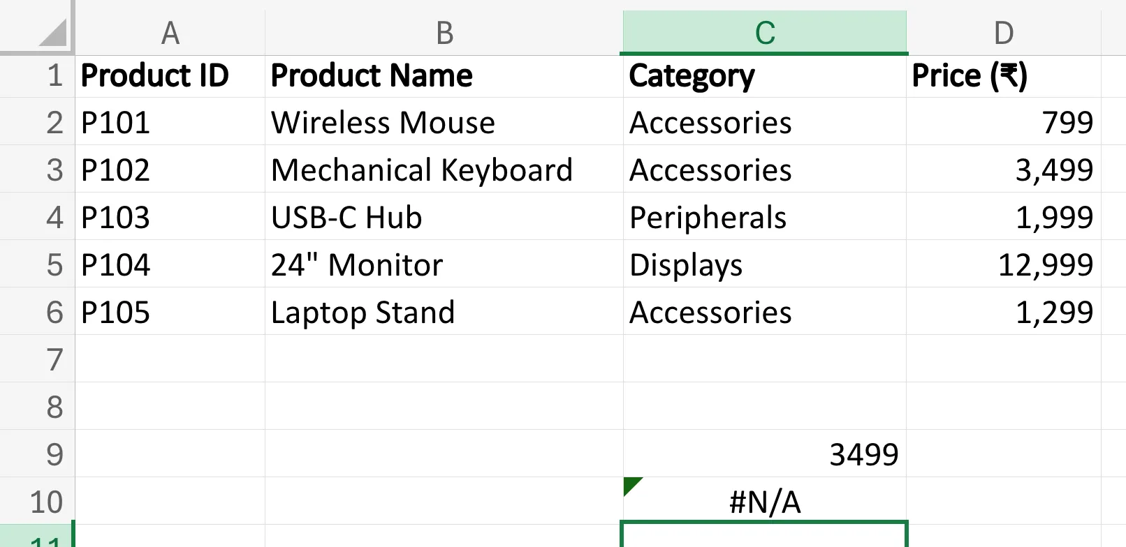
To avoid this, we add absolute references in the table_range. The correct formula then becomes:

=VLOOKUP(B3,$B$2:$D$6,3,FALSE)

So, to summarise, absolute references ensure your lookup table stays fixed. With that, you can scale your formula confidently across hundreds or thousands of rows.

But wait, there is another way to tackle relative referencing.

Using Excel Tables with VLOOKUP

While absolute references solve the shifting-range problem, there is an even smarter way to make your VLOOKUP formulas future-proof: Excel Tables.

When you convert your data range into a table, Excel automatically keeps track of the entire dataset. The dataset stays intact even when new rows are added or old ones are removed. This means your VLOOKUP formula continues to work without any manual updates.

Why is this useful?

Imagine that your warehouse list grows every week with new products. If your formula references a fixed range like $B$2:$D$6, you would need to update it every time the table expands. But if the data is stored in an Excel Table, the formula automatically includes the new entries.

How to convert data into a table

• Select your dataset.
• Press Ctrl + T (or go to Insert → Table).
• Confirm that your table has headers.
• Excel assigns a name such as Table1 (you can rename it later).
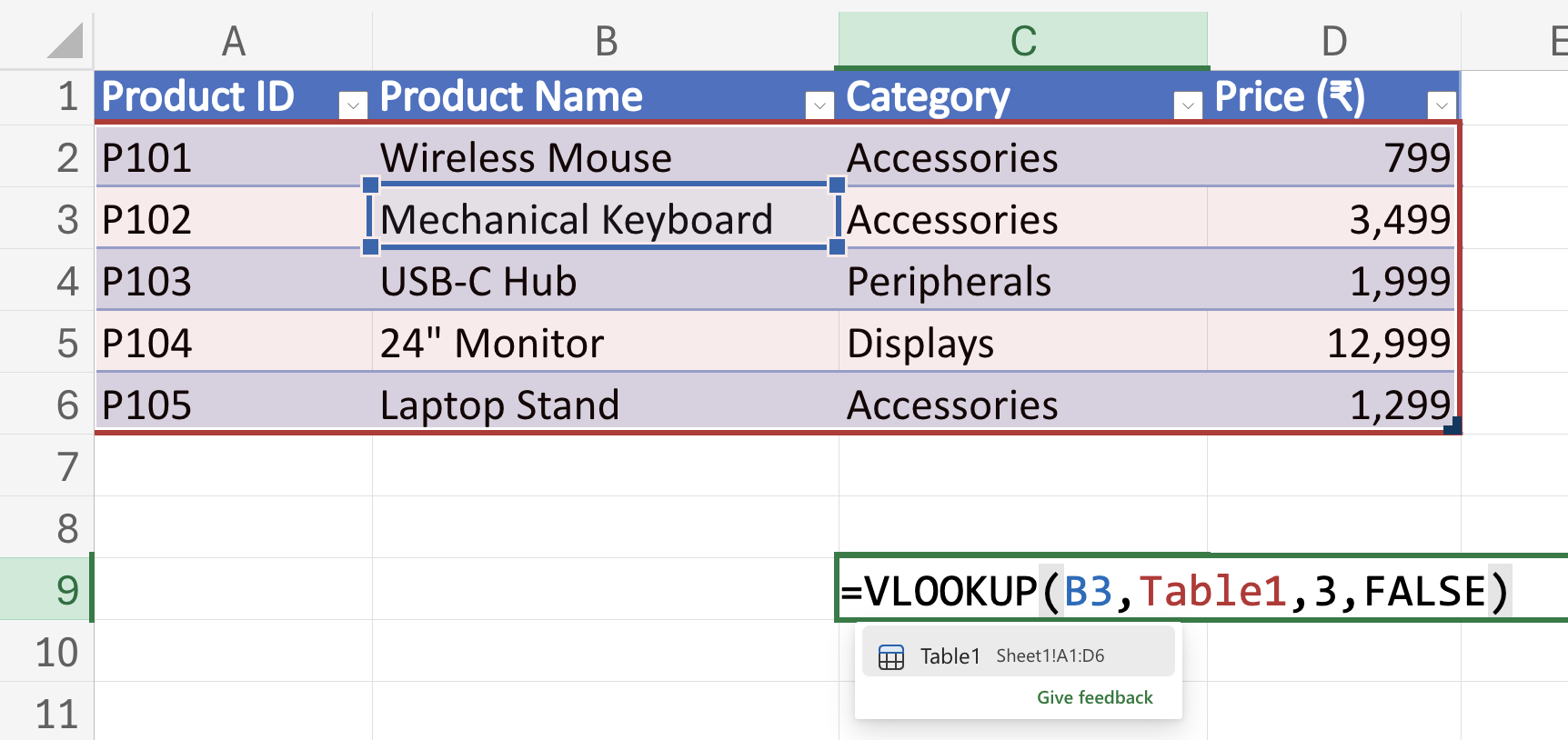
• Instead of a cell range, reference the table name:
  =VLOOKUP(B3,Table1,3,FALSE)

Now, whenever new rows are added to the table, the formula still works perfectly.

When should you use Excel Tables?

• Growing datasets (sales logs, inventory, customer lists)
• Dashboards that update regularly
• Reports that require frequent data additions
• Collaborative spreadsheets where the structure may change

In short, Excel Tables make your formulas smarter, more dynamic, and maintenance-free — exactly what you want when working with real-world data.

Also read: 50+ Excel Interview Questions to Ace Your Interview

Limitations of VLOOKUP

As powerful as VLOOKUP is, it is not perfect. Understanding its limitations will save you hours of confusion later. Here are some:

• Lookup value must be in the first column:
  VLOOKUP can only search left → right. If the value you need lies to the left, the formula won’t work.
• Single match only:
  It returns the first match it finds and not multiple results.
• Column numbers are static:
  If you insert or rearrange columns, the column index can break and return incorrect results.
• Not ideal for large datasets:
  On very large spreadsheets, VLOOKUP can slow performance.
• Approximate match pitfalls:
  If you forget to set FALSE, Excel defaults to an approximate match, which can produce wrong results.

Because of these limitations, modern Excel versions introduced XLOOKUP, a more flexible replacement that allows left lookups, dynamic columns, and more accurate matching.

That said, VLOOKUP remains one of the most widely used and essential functions you should master. Here are some pro tips to get the most out of it.

Pro Tips to Master VLOOKUP

If you want VLOOKUP to work smoothly every time (and avoid spreadsheet heartbreak), keep these expert tips in mind:

• Always use FALSE for exact matches:
  Exact match prevents incorrect results, especially when working with IDs, names, or codes.
• Lock your table range with absolute references:
  Press F4 to lock the range ($B$2:$D$100) before dragging the formula down.
• Use structured tables for dynamic data:
  Convert ranges into Excel Tables (Ctrl + T) so your formula auto-adjusts when data grows. Note, use either this or absolute references, not both.
• Double-check column index numbers:
  A wrong index returns wrong data. And Excel won’t warn you.
• Sort data when using TRUE (approximate match):
  Approximate match works correctly only when the lookup column is sorted in ascending order.
• Handle errors gracefully with IFERROR:
  The formula =IFERROR(VLOOKUP(…),”Not Found”) prevents ugly #N/A errors.
• Avoid duplicates in the lookup column:
  VLOOKUP returns the first match only. Duplicates can produce misleading results.
• Use helper columns when needed:
  Combine fields (e.g., ID + Date) to create unique lookup keys.

Master these small habits, and VLOOKUP will feel less like a formula and more like a superpower.

Conclusion

VLOOKUP has earned its reputation as one of Excel’s most powerful and widely used functions, and for good reason. As we just saw through examples, it completely eliminates tedious manual searching. Instead, it brings a fast, reliable process that can be scaled at will. Whether you work in finance, operations, HR, sales, or analytics, mastering VLOOKUP can save hours of effort and significantly reduce errors.

While newer functions like XLOOKUP offer added flexibility, VLOOKUP remains a foundational skill every Excel user should know. Learn it once, practise it with real datasets, and you’ll quickly realise why it continues to power spreadsheets across industries.

And yes! Here is the correct formula for the self-test exercise we did above:

=VLOOKUP(B6,B2:D6,3,False)