Introduction
Industry estimates that we are creating more than 2.5 Quintillion bytes of data every year.
Think of it for a moment – 1 Qunitillion = 1 Million Billion! Can you imagine how many drives / CDs / Blue-ray DVDs would be required to store them? It is difficult to imagine this scale of data generation even as a data science professional. While this pace of data generation is very exciting, it has created entirely new set of challenges and has forced us to find new ways to handle Big Huge data effectively.
Big Data is not a new phenomena. It has been around for a while now. However, it has become really important with this pace of data generation. In past, several systems were developed for processing big data. Most of them were based on MapReduce framework. These frameworks typically rely on use of hard disk for saving and retrieving the results. However, this turns out to be very costly in terms of time and speed.
On the other hand, Organizations have never been more hungrier to add a competitive differentiation through understanding this data and offering its customer a much better experience. Imagine how valuable would be Facebook, if it did not understand your interests well? The traditional hard disk based MapReduce kind of frameworks do not help much to address this challenge.
In this article, I will introduce you to one such framework, which has made querying and analysing data at a large scale much more efficient than previous systems / frameworks – Read on!
P.S. This article is meant for complete beginners on the topic and presumes minimal prior knowledge in Big Data
Table of Contents
- Challenges while working with Big Data
- Introduction to Distributed Computing Framework
- What is Apache Spark?
- History of Spark
- Common terms used
- Benefits of Spark over traditional big data frameworks
- Installation of Apache Spark (with Python)
- Python vs Scala
- Getting up to speed with RDD / Dataframe / Dataset
- Solving a machine learning problem
Challenges while working with big data
Challenges associated with big data can be classified in following categories:
- Challenges in data capturing: Capturing huge data could be a tough task because of large volume and high velocity. There are millions of sources emanating data at high speed. To deal with this challenge, we have created devices which can capture the data effectively and efficiently. For example, sensors which not only sense data like temperature of a room, steps count, weather parameters in real time, but send this information directly over to cloud for storage.
- Challenges with data storage: Given the increase in data generation, we need more efficient ways to store data. This challenge is typically dealt by combination of various methods including increasing disk sizes, compressing the data and using multiple machines, which are connected to each other and can share data efficiently.
- Challenges with Querying and Analysing data: This is probably the most difficult task at hand. The task is to not only to retrieve the past data, but also coming out with insights in real time (or as little time as possible). To handle this challenge, we can look at several options. One options is to increase the processing speed. However, this normally comes with increase in cost and can not scale as much. Alternately, we can build a network of machines or nodes known as “Cluster”. In this scenario, we first break a task to sub-tasks and distribute them to different nodes. At the end, we aggregate the output of each node to have final output. This distribution of task is known as “Distributed Computing”
Now that I have spoken of Distributed computing, let us get a bit deeper into it!
What is Distributing Computing Framework?
In simple terms, distributed computing is just a distributed system, where multiple machines are doing certain work at the same time. While doing the work, machines will communicate with each other by passing messages between them. Distributed computing is useful, when there is requirement of fast processing (computation) on huge data.
Let us take a simple analogy to explain the concept. Let us say, you had to count the number of books in various sections of a really large library. And you have to finish it in less than an hour. This number has to be exact and can not be approximated. What would you do? If I was in this position, I would call up as many friends as I can and divide areas / rooms among them. I’ll divide the work in non-overlapping manner and ask them to report back to be in 55 minutes. Once they come back, I’ll simply add up the numbers to come up with a solution. This is exactly how distributed computing works.
Apache Hadoop and Apache Spark are well-known examples of Big data processing systems. Hadoop and Spark are designed for distributed processing of large data sets across clusters of computers. Although, Hadoop is widely used for fast distributed computing, it has several disadvantages. For example, it does not use “In-memory computation“, which is nothing but keeping the data in RAM instead of Hard Disk for fast processing. In-memory computation enables faster processing of Big data. When Apache Spark was developed, it overcame this problem by using In-memory computation for fast computing.
MapReduce is also used widely, when the task is to process huge amounts of data, in parallel (more than one machines are doing a certain task at the same time), on large clusters. You can learn more about MapReduce from this link.
What is Apache Spark?
Apache Spark is a fast cluster computing framework which is used for processing, querying and analyzing Big data. It is based on In-memory computation, which is a big advantage of Apache Spark over several other big data Frameworks. Apache Spark is open source and one of the most famous Big data framework. It can run tasks up to 100 times faster, when it utilizes the in-memory computations and 10 times faster when it uses disk than traditional map-reduce tasks.
Please note that Apache Spark is not a replacement of Hadoop. It is actually designed to run on top of Hadoop.
History of Apache Spark
Apache Spark was originally created at University of California, Berkeley’s AMPLab in 2009. The Spark code base was later donated to the Apache Software Foundation. Subsequently, it was open sourced in 2010. Spark is mostly written in Scala language. It has some code written in Java, Python and R. Apache Spark provides several APIs for programmers which include Java, Scala, R and Python.
Key terms used in Apache Spark:
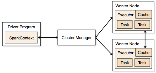
Image source: https://spark.apache.org/docs/1.1.1/img/cluster-overview.png
Spark Context: It holds a connection with Spark cluster manager. All Spark applications run as independent set of processes, coordinated by a SparkContext in a program.
Driver and Worker: A driver is incharge of the process of running the main() function of an application and creating the SparkContext. A worker, on the other hand, is any node that can run program in the cluster. If a process is launched for an application, then this application acquires executors at worker node.
Cluster Manager: Cluster manager allocates resources to each application in driver program. There are three types of cluster managers supported by Apache Spark – Standalone, Mesos and YARN. Apache Spark is agnostic to the underlying cluster manager, so we can install any cluster manager, each has its own unique advantages depending upon the goal. They all are different in terms of scheduling, security and monitoring. Once SparkContext connects to the cluster manager, it acquires executors on a cluster node, these executors are worker nodes on cluster which work independently on each tasks and interact with each other.
How Apache Spark is better than traditional big data framework?
In-memory computation: The biggest advantage of Apache Spark comes from the fact that it saves and loads the data in and from the RAM rather than from the disk (Hard Drive). If we talk about memory hierarchy, RAM has much higher processing speed than Hard Drive (illustrated in figure below). Since the prices of memory has come down significantly in last few years, in-memory computations have gained a lot of momentum.
Spark uses in-memory computations to speed up 100 times faster than Hadoop framework.

Image Source: https://en.wikipedia.org/wiki/Memory_hierarchy
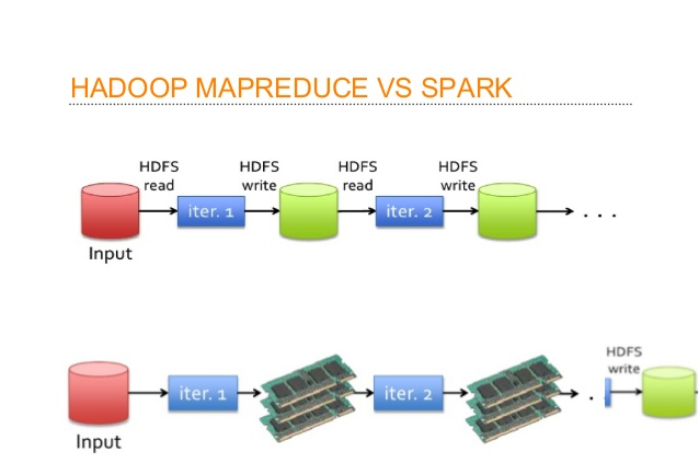
In Hadoop, tasks are distributed among the nodes of a cluster, which in turn save data on disk. When that data is required for processing, each node has to load the data from the disk and save the data into disk after performing operation. This process ends up adding cost in terms of speed and time, because disk operations are far slower than RAM operations. It also requires time to convert the data in a particular format when writing the data from RAM to disk. This conversion is known as Serialization and reverse is Deserialization.
Let’s look at the MapReduce process to understand the advantage of in-memory computation better. Suppose, there are several map-reduce tasks happening one after another. At the start of the computations, both technologies (Hadoop and Spark), read the data from disk for mapping. Hadoop performs the map operation and saves the results back to hard drive. However, in case of Apache Spark, the results are stored in RAM.
In the next step (Reduce operation), Hadoop reads the saved data from the hard drive, where as Apache Spark reads it from RAM. This creates a difference in a single MapReduce operation. Now imagine, if there were multiple map-reduce operations, how much time difference would you see at the end of task completion.
Language Support: Apache Spark has API support for popular data science languages like Python, R, Scala and Java.
Supports Real time and Batch processing: Apache Spark supports “Batch data” processing where a group of transactions is collected over a period of time. It also supports real time data processing, where data is continuously flowing from the source. For example, weather information coming in from sensors can be processed by Apache Spark directly.
Lazy operation: Lazy operations are used to optimize solutions in Apache Spark. I will discuss about lazy evaluation in later part of this article. For now, we can think that there are some operations which do not execute until we require results.
Support for multiple transformations and actions: Another advantage of Apache Spark over Hadoop is that Hadoop supports only MapReduce but Apache Spark support many transformations and actions including MapReduce.
There are further advantages of Apache Spark in comparison to Hadoop. For example, Apache Spark is much faster while doing Map side shuffling and Reduce side shuffling. However, shuffling is a complex topic in itself and requires an entire article in itself. Hence, I am not talking about it in more details here.
Installation of Apache Spark with PySpark
We can install Apache Spark in many different ways. Easiest way to install Apache Spark is to start with installation on a single machine. Again, we will have choices of different Operating Systems. For installing in a single machine, we need to have certain requirements fulfilled. I am sharing steps to install for Ubuntu (14.04) for Spark version 1.6.0. I am installing Apache Spark with Python which is known as PySpark (Spark Python API for programmer). If you are interested in the R API SparkR, have a look at this learning path.
OS: Ubuntu 14.04, 64 bit . (If you are running on Windows or Mac and are new to this domain, I would strongly suggest to create a Virtual Ubuntu machine with 4 GB RAM and follow the rest of the process).
Softwares Required: Java 7+, Python 2.6+, R 3.1+
Installation Steps:
Step 0: Open the terminal.
Step 1: Install Java
 $ sudo apt-add-repository ppa:webupd8team/java
 $ sudo apt-get update
 $ sudo apt-get install oracle-java7-installer
If you are asked to accept Java license terms, click on “Yes” and proceed. Once finished, let us check whether Java has installed successfully or not. To check the Java version and installation, you can type:
$ java -version
Step 2 : Once Java is installed, we need to install Scala
 $ cd ~/Downloads
 $ wget http://www.scala-lang.org/files/archive/scala-2.11.7.deb
 $ sudo dpkg -i scala-2.11.7.deb
 $ scala –version
This will show you the version of Scala installed
Step 3: Install py4j
Py4J is used on the driver for local communication between the Python and Java SparkContext objects; large data transfers are performed through a different mechanism.
$ sudo pip install py4j
Step 4: Install Spark.
By now, we have installed the dependencies which are required to install Apache Spark. Next, we need to download and extract Spark source tar. We can get the latest version Apache Spark using wget:
 $ cd ~/Downloads
 $ wget http://d3kbcqa49mib13.cloudfront.net/spark-1.6.0.tgz
 $ tar xvf spark-1.6.0.tgz
Step 5: Compile the extracted source
sbt is an open source build tool for Scala and Java projects which is similar to Java’s Maven.
 $ cd ~/Downloads/spark-1.6.0
 $ sbt/sbt assembly
This will take some time to install Spark. After installing, we can check whether Spark is running correctly or not by typing.
$ ./bin/run-example SparkPi 10
this will produce the output:
Pi is roughly 3.14042
To see the above results we need to lower the verbosity level of the log4j logger in log4j.properties.
$ cp conf/log4j.properties.template conf/log4j.properties
$ nano conf/log4j.properties
After opening the file ‘log4j.properties’, we need to replace following line:
log4j.rootCategory=INFO, console
log4j.rootCategory=ERROR, console
Step 6: Move the files in the right folders (to make it convenient to access them)
$ sudo mv ~/Downloads/spark-1.6.0 /opt/
$ sudo ln -s /opt/spark-1.6.0 /opt/spark
Add this to your path by editing your bashrc file:
Step 7: Create environment variables. To set the environment variables, open bashrc file in any editor.
$ nano ~/.bashrc
Set the SPARK_HOME and PYTHONPATH by adding following lines at the bottom of this file
export SPARK_HOME=/opt/spark
export PYTHONPATH=$SPARK_HOME/python
Next, restart bashrc by typing in:
$ . ~/.bashrc
Let’s add this setting for ipython by creating a new python script to automatically export settings, just in case above change did not work.
$ nano ~/.ipython/profile_default/startup/load_spark_environment_variables.py
Paste some lines in this file.
import os
import sys

if 'SPARK_HOME' not in os.environ:
    os.environ['SPARK_HOME'] = '/opt/spark'

if '/opt/spark/python' not in sys.path:
    sys.path.insert(0, '/opt/spark/python')
Step 8: We are all set now. Let us start PySpark by typing command in root directory:
$ ./bin/pyspark --packages
We can also start ipython notebook in shell by typing:
$ PYSPARK_DRIVER_PYTHON=ipython ./bin/pyspark
When we launch the shell in PySpark, it will automatically load spark Context as sc and SQLContext as sqlContext.
Python vs Scala:
One of the common question people ask is whether it is necessary to learn Scala to learn Spark? If you are some one who already knows Python to some extent or are just exploring Spark as of now, you can stick to Python to start with. However, if you want to process some serious data across several machines and clusters, it is strongly recommended that you learn Scala. Computation speed in Python is much slower than Scala in Apache Spark.
- Scala is native language for Spark (because Spark itself written in Scala).
- Scala is a compiled language where as Python is an interpreted language.
- Python has process based executors where as Scala has thread based executors.
- Python is not a JVM (java virtual machine) language.
Apache Spark data representations: RDD / Dataframe / Dataset
Spark has three data representations viz RDD, Dataframe, Dataset. For each data representation, Spark has a different API. For example, later in this article I am going to use ml (a library), which currently supports only Dataframe API. Dataframe is much faster than RDD because it has metadata (some information about data) associated with it, which allows Spark to optimize query plan. Refer to this link to know more about optimization. The Dataframe feature in Apache Spark was added in Spark 1.3. If you want to know more in depth about when to use RDD, Dataframe and Dataset you can refer this link.
In this article, I will first spend some time on RDD, to get you started with Apache Spark. Later, I will spend some time on Dataframes. Dataframes share some common characteristics with RDD (transformations and actions). In this article, I am not going to talk about Dataset as this functionality is not included in PySpark.
RDD:
After installing and configuring PySpark, we can start programming using Spark in Python. But to use Spark functionality, we must use RDD. RDD (Resilient Distributed Database) is a collection of elements, that can be divided across multiple nodes in a cluster to run parallel processing. It is also fault tolerant collection of elements, which means it can automatically recover from failures. RDD is immutable, we can create RDD once but can’t change it. We can apply any number of operation on it and can create another RDD by applying some transformations. Here are a few things to keep in mind about RDD:
We can apply 2 types of operations on RDDs:
Transformation: Transformation refers to the operation applied on a RDD to create new RDD.
Action: Actions refer to an operation which also apply on RDD that perform computation and send the result back to driver.
Example: Map (Transformation) performs operation on each element of RDD and returns a new RDD. But, in case of Reduce (Action), it reduces / aggregates the output of a map by applying some functions (Reduce by key). There are many transformations and actions are defined in Apache Spark documentation, I will discuss these in a later article.
RDDs use Shared Variable:
The parallel operations in Apache Spark use shared variable. It means that whenever a task is sent by a driver to executors program in a cluster, a copy of shared variable is sent to each node in a cluster, so that they can use this variable while performing task. Accumulator and Broadcast are the two types of shared variables supported by Apache Spark.
Broadcast: We can use the Broadcast variable to save the copy of data across all node.
Accumulator: In Accumulator variables are used for aggregating the information.
How to Create RDD in Apache Spark
Existing storage: When we want to create a RDD though existing storage in driver program (which we would like to be parallelized). For example, converting a list to RDD, which is already created in a driver program.
External sources: When we want to create a RDD though external sources such as a shared file system, HDFS, HBase, or any data source offering a Hadoop Input Format.
Writing first program in Apache Spark
I have already discussed that RDD supports two type of operations, which are transformation and action. Let us get down to writing our first program:
Step1: Create SparkContext
First step in any Apache programming is to create a SparkContext. SparkContext is needed when we want to execute operations in a cluster. SparkContext tells Spark how and where to access a cluster. It is first step to connect with Apache Cluster. If you are using Spark Shell, we will find that this is already created. Otherwise, we can create the Spark Context by importing, initializing and providing the configuration settings. For example:
 from pyspark import SparkContext
 sc = SparkContext()
Step2: Create a RDD
I have already discussed that we can create RDD in two ways: Either from an existing storage or from an external storage. Let’s create our first RDD. SparkContext has parallelize method, which is used for creating the Spark RDD from an iterable (like list, tuple..) already present in driver program.
We can also provide the number of partitions as a parameter to parallelize method. If we do not give number of partition parameter, then Spark will automatically set the number of partition in a cluster. The number of partition can be set manually by passing second parameter to parallelize method. For example, sc.parallelize(data, 10)), where data is an existing data in driver program and 10 is the number of partitions.
Lets create the first Spark RDD called rdd.
data = range(1,1000)
rdd = sc.parallelize(data)
We have a collect method to see the content of RDD.
rdd.collect()
To see the first n element of a RDD we have a method take:
rdd.take(2) # It will print first 2 elements of rdd
We have 2 parallel operations in RDD which are Transformation and Action. Transformation and Action were already discussed briefly earlier. So let’s see how transformation works. Remember that RDDs are immutable – so we can’t change our RDD, but we can apply transformation on it. Let’s see an example of map transformation to demonstrate how transformation works.
Step 3: Map transformation.
Map transformation returns a Mapped RDD by applying function to each element of the base RDD. Let’s repeat the first step of creating a RDD from existing source, For example,
data = ['Hello' , 'I' , 'AM', 'Ankit ', 'Gupta']
Rdd = sc.parallelize(data)
Now a RDD (name is ‘Rdd’) is created from the existing source, which is a list of string in a driver program. We will now apply lambda function to each element of Rdd and return the mapped (transformed) RDD (word,1) pair in the Rdd1.
Rdd1 = Rdd.map(lambda x: (x,1))
Let’s see the out of this map operation.
Rdd1.collect()
output: [('Hello', 1), ('I', 1), ('AM', 1), ('Ankit ', 1), ('Gupta', 1)]
If you noticed, nothing happened after applying the lambda function on Rdd1 (we won’t see any computation happening in a cluster). This is called the lazy operation. All transformation operations in Spark are lazy, which means that we will not see any computations on RDD, until we need them for further action.
Spark remembers which transformation is applied to which RDD with the help of DAG (Directed a Cyclic Graph). The lazy evaluation helps Spark to optimize the solution because Spark will get time to see the DAG before actually executing the operations on RDD. This enables Spark to run operations more efficiently.
In the code above, collect() and take() are the examples of an action.
There are many number of transformation defined in Apache Spark. We will talk more about them in a future post.
Solving a machine learning problem:
We have covered a lot of ground already. We started with understanding what Spark brings to the table, its data representations, installed Spark and have already played with our first RDD. Now, I’ll demonstrate solution to “Practice Problem: Black Friday” using Apache Spark. Even if you don’t understand these commands completely as of now, it is fine. Just follow along, we will take them up again in a future tutorial.
Let’s look at the steps:
Reading a data file (csv)
For reading the csv file in Apache Spark, we need to specify the library in python shell. Lets read the the data from a csv files to create the Dataframe and apply some data science skills on this Dataframe like we do in Pandas.
For reading the csv file, first we need to download Spark-csv package (Latest) and extract this package into the home directory of Spark. Then, we need to open a PySpark shell and include the package (I am using “spark-csv_2.10:1.3.0”).
$ ./bin/pyspark --packages com.databricks:spark-csv_2.10:1.3.0
In Apache Spark, we can read the csv file and create a Dataframe with the help of SQLContext. Dataframe is a distributed collection of observations (rows) with column name, just like a table. Let’s see how can we do that.
Please note that since I am using pyspark shell, there is already a sparkContext and sqlContext available for me to use. In case, you are not using pyspark shell, you might need to type in the following commands as well:
sc = sparkContext()
sqlContext = SQLContext(sc)
First download the train and test file and load these with the help of SparkContext
train = sqlContext.load(source="com.databricks.spark.csv", path = 'PATH/train.csv', header = True,inferSchema = True)
test = sqlContext.load(source="com.databricks.spark.csv", path = 'PATH/test-comb.csv', header = True,inferSchema = True)
PATH is the location of folder, where your train and test csv files are located. Header is True, it means that the csv files contains the header. We are using inferSchema is True for telling sqlContext to automatically detect the data type of each column in data frame. If we do not set inferSchema to true, all columns will be read as string.
Analyze the data type
To see the types of columns in Dataframe, we can use the method printSchema(). Lets apply printSchema() on train which will Print the schema in a tree format.
train.printSchema()
Previewing the data set
To see the first n rows of a Dataframe, we have head() method in PySpark, just like pandas in python. We need to provide an argument (number of rows) inside the head method. Lets see first 10 rows of train:
train.head(10)
To see the number of rows in a data frame we need to call a method count(). Lets check the number of rows in train. The count method in pandas and Spark are different.
train.count()
Impute Missing values
We can check number of not null observations in train and test by calling drop() method. By default, drop() method will drop a row if it contains any null value. We can also pass ‘all” to drop a row only if all its values are null.
train.na.drop().count(),test.na.drop('any').count()
Here, I am imputing null values in train and test file with -1. Imputing the values with -1 is not an elegant solution. We have several algorithms / techniques to impute null values, but for the simplicity I am imputing null with constant value (-1). We can transform our base train, test Dataframes after applying this imputation. For imputing constant value, we have fillna method. Lets fill the -1 in-place of null in all columns.
train = train.fillna(-1)
test = test.fillna(-1)
Analyzing numerical features
We can also see the various summary Statistics of a Dataframe columns using describe() method, which shows statistics for numerical variables. To show the results we need to call show() method.
train.describe().show()
Sub-setting Columns
Let’s select a column called ‘User_ID’ from a train, we need to call a method ‘select’ and pass the column name which we want to select. The select method will show result for selected column. We can also select more than one column from a data frame by providing columns name separated by comma.
train.select('User_ID').show()
Analyzing categorical features
To start building a model, we need to see the distribution of categorical features in train and test. Here I am showing this for only Product_ID but we can also do the same for any categorical feature. Let’s see the number of distinct categories of “Product_ID” in train and test. Which we can do by applying methods distinct() and count().
train.select('Product_ID').distinct().count(), test.select('Product_ID').distinct().count()
Output:(3631, 3491)
After counting the number of distinct values for train and test we can see the train has more categories than test. Let us check what are the categories for Product_ID, which are in test but not in train by applying subtract method.We can also do the same for all categorical feature.
diff_cat_in_train_test=test.select('Product_ID').subtract(train.select('Product_ID'))
diff_cat_in_train_test.distinct().count()# For distict count
Output: 46
Above you can see that 46 different categories are in test not in train. In this case, either we collect more data about them or skip the rows in test for those categories(invalid category) which are not in train.
Transforming categorical variables to labels
We also need to transform categorical columns to label by applying StringIndexer Transformation on Product_ID which will encode the Product_ID column of labels to a column of label indices. You can see more about this from the link
from pyspark.ml.feature import StringIndexer
plan_indexer = StringIndexer(inputCol = 'Product_ID', outputCol = 'product_ID')
labeller = plan_indexer.fit(train)
Above, we build a ‘labeller’ by applying fit() method on train Dataframe. Later we will use this ‘labeller’ to transform our train and test. Let us transform our train and test Dataframe with the help of labeller. We need to call transform method for doing that. We will store the transformation result in Train1 and Test1.
Train1 = labeller.transform(train)
Test1 = labeller.transform(test)
Lets check the resulting Train1 Dataframe.
Train1.show()
The show method on Train1 Dataframe will show that we successfully added one transformed column product_ID in our previous train Dataframe.
Selecting Features to Build a Machine Learning Model
Let’s try to create a formula for Machine learning model like we do in R. First, we need to import RFormula from the pyspark.ml.feature. Then we need to specify the dependent and independent column inside this formula. We also have to specify the names for features column and label column.
from pyspark.ml.feature import RFormula
formula = RFormula(formula="Purchase ~ Age+ Occupation +City_Category+Stay_In_Current_City_Years+Product_Category_1+Product_Category_2+ Gender",featuresCol="features",labelCol="label")
After creating the formula we need to fit this formula on our Train1 and transform Train1,Test1 through this formula. Lets see how to do this and after fitting transform train1,Test1 in train1,test1.
t1 = formula.fit(Train1)
train1 = t1.transform(Train1)
test1 = t1.transform(Test1)
We can see the transformed train1, test1.
train1.show()
After applying the formula we can see that train1 and test1 have 2 extra columns called features and label those we have specified in the formula (featuresCol=”features” and labelCol=”label”). The intuition is that all categorical variables in the features column in train1 and test1 are transformed to the numerical and the numerical variables are same as before for applying ML. Purchase variable will transom to label column. We can also look at the column features and label in train1 and test1.
train1.select('features').show()
train1.select('label').show()
Building a Machine Learning Model: Random Forest
After applying the RFormula and transforming the Dataframe, we now need to develop the machine learning model on this data. I want to apply a random forest regressor for this task. Let us import a random forest regressor, which is defined in pyspark.ml.regression and then create a model called rf. I am going to use default parameters for randomforest algorithm.
from pyspark.ml.regression import RandomForestRegressor
rf = RandomForestRegressor()
After creating a model rf we need to divide our train1 data to train_cv and test_cv for cross validation.
Here we are dividing train1 Dataframe in 70% for train_cv and 30% test_cv.
(train_cv, test_cv) = train1.randomSplit([0.7, 0.3])
Now build the model on train_cv and predict on test_cv. The results will save in predictions.
model1 = rf.fit(train_cv)
predictions = model1.transform(test_cv)
If you check the columns in predictions Dataframe, there is one column called prediction which has prediction result for test_cv.
model1 = rf.fit(train_cv)
predictions = model1.transform(test_cv)
Lets evaluate our predictions on test_cv and see what is the mean squae error.
To evaluate model we need to import RegressionEvaluator from the pyspark.ml.evaluation. We have to create an object for this. There is a method called evaluate for evaluator which will evaluate the model. We need to specify the metrics for that.
from pyspark.ml.evaluation import RegressionEvaluator
evaluator = RegressionEvaluator()
mse = evaluator.evaluate(predictions,{evaluator.metricName:"mse" })
import numpy as np
np.sqrt(mse), mse
After evaluation we can see that our root mean square error is 3773.1460883883865 which is a square root of mse.
Now, we will implement the same process on full train1 dataset.
model = rf.fit(train1)
predictions1 = model.transform(test1)
After prediction, we need to select those columns which are required in Black Friday competition submission.
df = predictions1.selectExpr("User_ID as User_ID", "Product_ID as Product_ID", 'prediction as Purchase')
Now we need to write the df in csv format for submission.
df.toPandas().to_csv('submission.csv')
After writing into the csv file(submission.csv). We can upload our first solution to see the score, I got the score 3822.121053 which is not very bad for first model out of Spark!
End Note:
In this article, I introduced you to the fascinating world of Apache Spark. This is only the start of things to come in this series. In the next few weeks, I will continue to share tutorials for you to master the use of Apache Spark. If this article feels like a lot of work, it is! So, take your time and digest this comprehensive guide.
In the meanwhile, if you have any questions or you want to give any suggestions on what I should cover, feel free to drop them in the notes below.
Ankit is currently working as a data scientist at UBS who has solved complex data mining problems in many domains. He is eager to learn more about data science and machine learning algorithms.


hello i want some suggestions.which language i should use for weather analysis . as i want to implement it on spark .should i use R or python or FORTRAN? or any other ?? i am using hdf5 file format images..
Hi Urmay, Python is a general-purpose programming language but R is mostly use by data scientist. It is tough to say that which language would be a batter option because each has it's unique advantages. The Fortran API is not availible in Apache spark. Regards Ankit
Nice Tutorial. You have installed scala too in between . Is it required if we are using python, i.e. pySpark.
Installing Scala is compulsory to install Apache Spark because Apache Spark has dependency on Scala.
Thank you Ankit, good article, very clear ! What about create a new layer on the Docker Kaggle/Python2 for SpySpark ? Or better what about write an article to how to create a new layer on an existing Docker Image ? Thank you Ankit keep going this way !