Part 7: Step by Step Guide to Master NLP – Word Embedding in Detail

This article was published as a part of the Data Science Blogathon

Introduction

This article is part of an ongoing blog series on Natural Language Processing (NLP). In the previous articles (part-5 and 6), we completed the different text vectorization and word embeddings techniques in detail. In this article, firstly we will discuss the co-occurrence matrix, which is also a word vectorization technique and after that, we will be discussing new concepts related to the Word embedding that includes,

• Applications of Word Embeddings,
• Word Embedding use-cases,
• Implementation of word embedding using a pre-trained model and also from scratch.

This is part-7 of the blog series on the Step by Step Guide to Natural Language Processing.

Table of Contents

1. Distributional Similarity-based Word Representations

2. Co-occurrence matrix with a fixed context window

• Different variations of the co-occurrence matrix
• Advantages and disadvantages of the co-occurrence matrix

3. Applications of Word Embedding

4. Word Embedding use case Scenarios

5. Word embedding using Pre-trained Word Vectors

6. Training your own Word Vectors

Distributional Similarity-based Word Representations

The big idea behind this – You can get a lot of value by representing a word by means of its neighbors.

But the question that comes to mind is,

How to make Neighbors Represent Words?

The answer to the above question is to use a Co-occurrence matrix X.

We have 2 options in hand – either use full document or windows. Let’s discuss these 2 methods one by one:

If we use Word – document co-occurrence matrix, then it will give an idea about the general topics (like all sports terms will have similar entries) which leads to “Latent Semantic Analysis”.

Instead, if we used Window around each word, it will capture both syntactic (POS) and semantic information. So, we use the window concept for our later discussion.

Now, let’s discuss the co-occurrence matrix with a fixed context window in the next section.

Co-Occurrence Matrix with a fixed context window

The big idea about the concept:

• Similar words tend to occur together and will have similar contexts
• Window length 1 (more common: 5 – 10)
• Symmetric (irrelevant whether left or right context)

Let’s consider the following examples for a better understanding:

Example-1: Consider the following sentences:

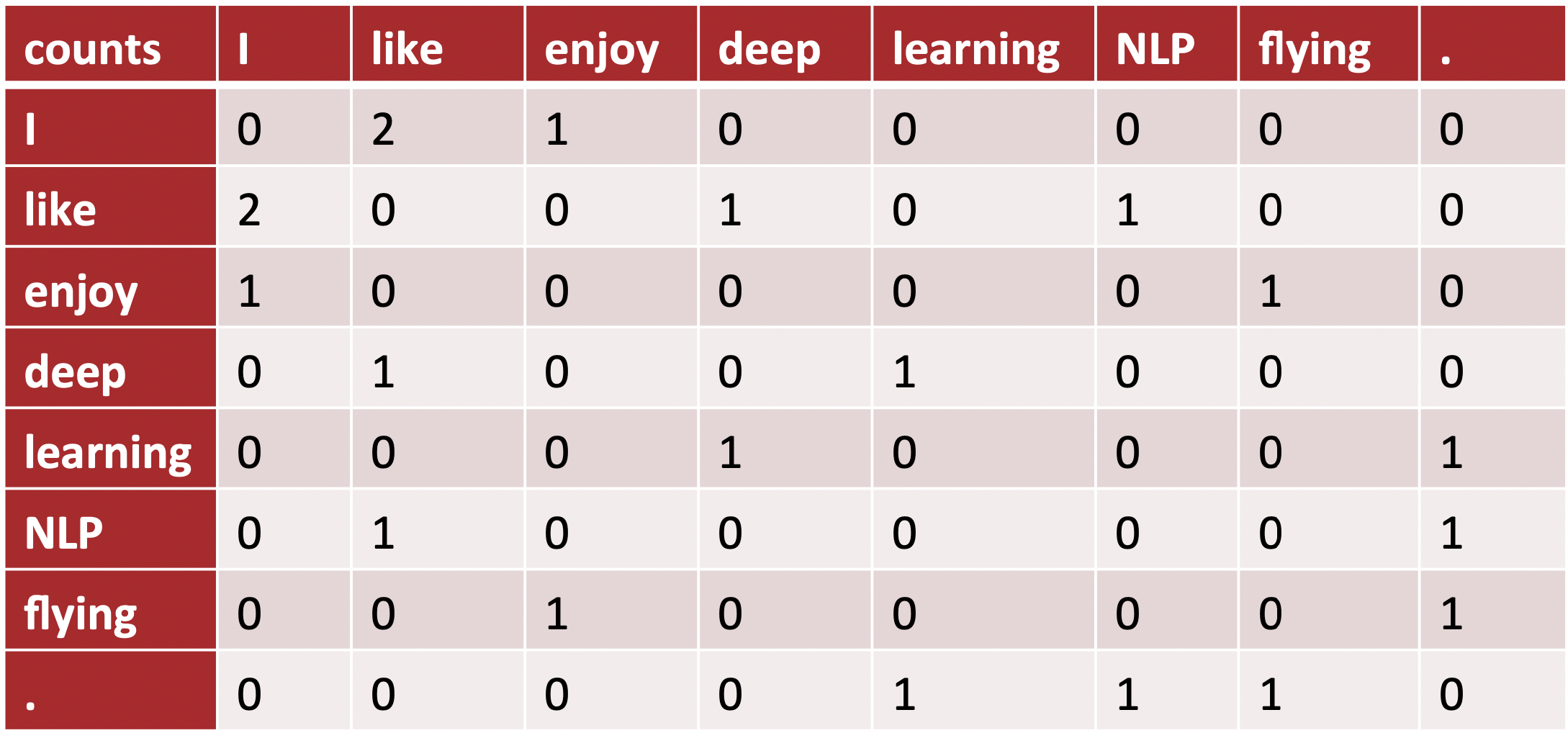
Example Corpus: I like deep learning. I like NLP. I enjoy flying.

From the above corpus, the list of unique words present are as follows:

Dictionary: [ 'I', 'like', 'enjoy', 'deep', 'learning', 'NLP', 'flying', '.' ]

The co-occurrence matrix for the above corpus becomes:

Example-2: Consider the following sentence:

Example Corpus: Apple is a fruit. Mango is a fruit.

In the above sentence, Apple and mango tend to have a similar context i.e fruit.

Before we deep dive into the details of the construction of the co-occurrence matrix, there are two concepts that you have to understand properly

• Co-Occurrence
• Context Window

Co-occurrence

For a given set of documents i.e, corpus, the co-occurrence of a pair of words say x1 and x2 are equal to the frequency (the number of times) the two words have appeared together in a Context Window.

Context Window

The context window is specified with the help of a number and the direction. Let’s consider the following example, to understand what does a context window of 2(around) represents?

Sentence: Quick Brown Fox Jump Over The Lazy Dog

The green words are a 2 (around) context window for the word ‘Fox’ and only these green words are used for calculating the co-occurrence. Let us see the context window for the word ‘Over’.

Now, let us consider the following example of corpus to compute a co-occurrence matrix.

Corpus:  He is not lazy. He is intelligent. He is smart.

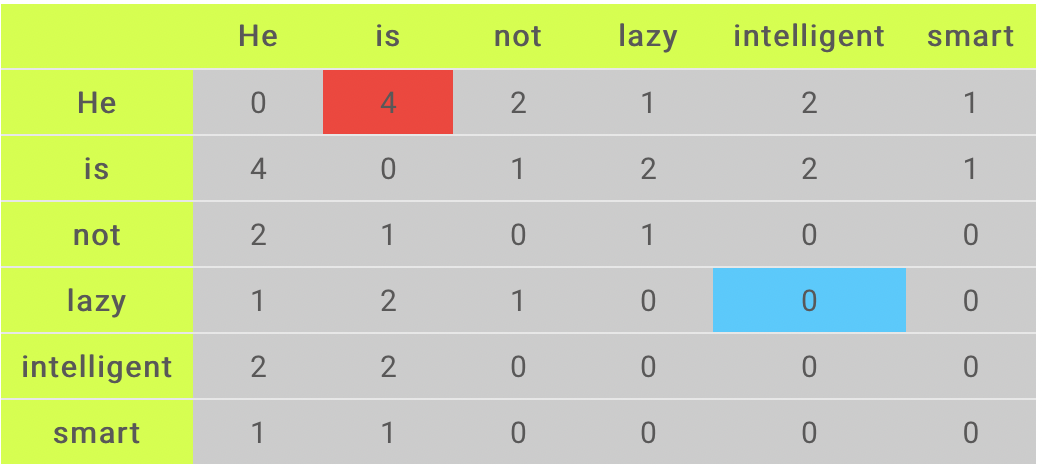
                                                  Image Source: Google Images

From the corpus, we can form our dictionary i.e, a list of unique words in the following way:

Unique Words: [ ‘He’, ‘is’, ‘not’, ‘lazy’, ‘intelligent’, ‘smart’ ]

To understand the above co-occurrence matrix properly, we focused our discussion on the two cells shown in the above matrix – Red and the blue cells.

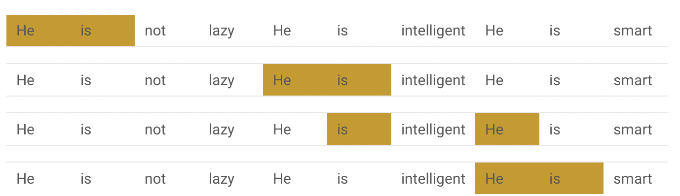
Red cell: This cell indicates the number of times the words ‘He’ and ‘is’ have appeared in the context window 2 and here we have observed that the count of this is 4. To understand and visualize the count, the below table will help you.

Blue cell: The count of this cell is 0 since the word ‘lazy’ has never come with ‘intelligent’ in the context window of 2.

Problems with simple Co-occurrence vectors

• Increase in size with dictionary or vocabulary.
• Very high dimensional: require a lot of storage to store the matrix and subsequent classification models face the issue of sparsity.
• Models are less robust.

Solution: Low dimensional vectors

• Idea: We only store “most” of the important information in a fixed, small number of dimensions that is a  dense vector instead of a sparse vector.
• The dimension size is usually around 25 – 1000.

How to reduce dimensionality?

• Apply Dimensionality reduction on co-occurrence matrix X.
• Apply Singular Value Decomposition (SVD) Technique on co-occurrence matrix X.

Some Variations of the Co-occurrence Matrix

Let’s say we have K unique words present in the corpus. So dictionary size = K.

Since the columns of the Co-occurrence matrix form the context words, therefore, the different variations of the Co-Occurrence Matrix are as follows:

• A co-occurrence matrix of size K X K. Now, for even a decent corpus K that becomes very large and difficult to handle. So in general we cannot prefer this architecture in practice.
• A co-occurrence matrix of size K X N where N is a subset of K and can be obtained by removing irrelevant words like stopwords etc. But at this time also this becomes still very large, so we also face computational difficulties.

But, we have to note that this co-occurrence matrix is not the word vector representation that generally used. Instead, as we discussed in the above part we decompose this Co-occurrence matrix using techniques like Principal Component Analysis (PCA), Singular Value Decomposition (SVD), etc. into factors, and a combination of these factors will forms the word vector representation.

Let’s discuss the above idea more clearly:

For example, when we perform PCA on the above matrix of size K X K. We will obtain K principal components. We can choose y components out of these K components. So, the new matrix will be of the form K X y.

And, a single word, instead of being represented in K dimensions will be represented in y dimensions while still capturing almost the same semantic meaning. y is generally of the order of hundreds.

So, what PCA does at the back is decompose the Co-Occurrence matrix into three matrices, U, S, and V where U and V are both orthogonal matrices. What is of importance is that the dot product of U and S gives the word vector representation and V gives the word context representation.

Advantages of Co-occurrence Matrix

1. It preserves the semantic relationship between words.

For Example, man and woman tend to be closer than man and apple.

2. It uses Singular Value Decomposition (SVD) at its core, which produces more accurate word vector representations than existing methods.

3. It uses factorization which is a well-defined problem and can be efficiently solved.

4. If we compute this matrix once, then it can be used anytime wherever required. So, In this sense, it is faster than others.

Disadvantages of Co-Occurrence Matrix

To store the co-occurrence matrix, we require a huge amount of memory. But, to resolve this problem we can factorize the matrix out of the system.

Applications of Word Embedding 

The primary use of word embedding is to determining similarity, either in meaning or in usage. Usually, the computation of Similarity is done with the help of a metric such as the Cosine Similarity (i.e, a normalized dot product), between two vectors.

If our embedding model was trained properly, then similar words like storm and gale will show a high cosine similarity, as measured on a scale from 0 to 1.

Challenges for Word Embedding Models

However, we need to take care while we use the word embeddings. When we trained Embeddings using the contextual similarity model that is popularized with the help of models such as Word2Vec can often exhibit peculiarities that are surprising at first glance, although that makes complete sense while we go for further investigation into the method from which the model was trained.

For Example, Consider the following two words:

Words: Love and Hate

When we apply the cosine similarity metric on the above words, this will likely show high similarity, despite these words are having semantically opposite meanings. The reason behind high similarity since the contexts in which “love” is used is highly correlated with those in which “hate” is used. As such, the model categorizes them into the same category, despite the opposite meanings.

To mitigate the above challenges, by paying careful attention to the training procedure, there are some ways but we can also view that as a useful feature of the model, depending on how one decides to use the outputs.

Nearest Neighbors and Clustering

Some other use cases for word embeddings are as follows:

• Nearest neighbors
• Clustering methods, etc.

Let’s consider the following examples:

• In many use cases, we want to create topic models in which we cluster the words associated with a given topic.
• Also, we also find synonyms or substitutions for a given word by finding its nearest neighbors measured with the help of cosine similarity.

In both the mentioned instances, the semantic meaning encoded in the word representations allows one to use classic clustering and nearest neighbors methods such as k-means or KNN algorithms without much modification in order to produce a useful result.

Word Embeddings Use Case Scenarios

Since word embedding, which is also known as word Vectors represents the numerical representations of contextual similarities between words, therefore they can be manipulated and then used to perform some amazing tasks. Some of them are as follows

1. To Find the degree of similarity between two words

model.similarity('woman','man')
#Output
0.73723527

2. To Find the odd one out from a set of words

model.doesnt_match('breakfast cereal dinner lunch';.split())
#Output
'cereal'

3. Doing algebraic manipulations using the word (like Woman+King-Man =Queen)

model.most_similar(positive=['woman','king'],negative=['man'],topn=1)
#Output
queen: 0.508

4. To find the Probability of a text under the model

model.score(['The fox jumped over the lazy dog'.split()])
#Output
0.21

5. Can be used to perform Machine Translation

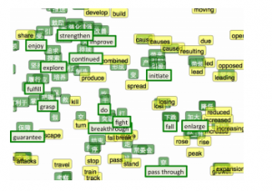
                                       Image Source: Google Images

The above graph represents a bilingual embedding with Chinese indicates with green color and English indicates in yellow color. Therefore, from this, if we know the words that are having similar meanings in Chinese and English, then the above bilingual embedding helps us to translate one language into the other.

Word Embedding Using pre-trained Word Vectors

To use word embedding with the help of pre-trained word vectors, here we are going to use google’s pre-trained model. Some of the details of this model are as follows:

• This model contains word vectors for a vocabulary of 3 million words that are trained on around 100 billion words collected from the google news dataset.
• If you want to download the model, then refer to this link. Here we have to take the precaution that the download is 1.5 GB, so you have to connect with a proper internet connection.

Let’s see all the steps one by one to use the Pre-trained model:

Step-1: Import Word2Vec from Gensim Library

from gensim.models import Word2Vec

Step-2: Loading the downloaded model

model = Word2Vec.load_word2vec_format('GoogleNews-vectors-negative300.bin', binary=True, norm_only=True)

# The model is loaded. It can be used to perform all of the tasks mentioned above.

Step-3: Getting word vectors of a word

dog = model['dog']

Step-4: Performing king queen magic

print(model.most_similar(positive=['woman', 'king'], negative=['man']))

Step-5: Picking odd one out

print(model.doesnt_match("breakfast cereal dinner lunch".split()))

Step-6: Printing similarity index

print(model.similarity('woman', 'man'))

Training your own Word Vectors

We can also train our own word2vec model on a custom corpus. For training that custom model we will be using the gensim library and all the included steps is described below:

As we know that the word2Vec requires a format of a list of lists for training where every document is contained in a list and every list contains a list of tokens of that documents. Here we do not cover the preprocessing steps since we covered all those techniques in our previous blogs, so if you want to see those please refer to our previous articles.

Now, Let’s take an example list of lists to train our word2vec model.

sentence: [ [‘Chirag’, ’ Boy’], [‘Kshitiz', ’ is’], [‘good’, ’ boy’]] 

Training word2vec on 3 sentences

model = gensim.models.Word2Vec(sentence, min_count=1,size=300,workers=4)

Let’s discuss the parameters of the above model for more clarity of the concept.

• sentence: Describes the list of our corpus.
• min_count: (1 – the threshold value for the words). We will include those words in the model for which the frequency is greater than the min_count.
• size: (300 – the number of dimensions in which we want to represent our word). This represents the size of the word vector.
• workers: (4 – used for parallelization).

Using the model

#The newly trained model can be used similar to the pre-trained ones.

Printing similarity index

print(model.similarity('woman', 'man'))

This ends our Part-7 of the Blog Series on Natural Language Processing!

Other Blog Posts by Me

You can also check my previous blog posts.

Previous Data Science Blog posts.

LinkedIn

Here is my Linkedin profile in case you want to connect with me. I’ll be happy to be connected with you.

Email

For any queries, you can mail me on Gmail.

End Notes

Thanks for reading!

I hope that you have enjoyed the article. If you like it, share it with your friends also. Something not mentioned or want to share your thoughts? Feel free to comment below And I’ll get back to you. 😉

The media shown in this article are not owned by Analytics Vidhya and are used at the Author’s discretion.

CHIRAG GOYAL 22 Jun 2021

I am currently pursuing my Bachelor of Technology (B.Tech) in Computer Science and Engineering from the Indian Institute of Technology Jodhpur(IITJ). I am very enthusiastic about Machine learning, Deep Learning, and Artificial Intelligence. Feel free to connect with me on Linkedin.