Numpy -Slicing and Dicing: A Beginner’s Guide

This article was published as a part of the Data Science Blogathon

Introduction :

Numpy is a package for scientific calculation in Python. It’s a ndarray under the hood and provides support for various mathematical operations such as basic linear algebra, basic linear statistics. Sklearn, pandas packages are built on top of numpy, and the transformation and manipulation operations work on the base numpy ndarrays. Numpy is the foundation on which a sizable chunk of data science stack is built on python. Below are a few use cases and instances to support my claim.

Table of Content :

1. Demonstration of numpy with an example.
2. Numpy is Faster than a python list.
3. Numpy hands on.
4. Numpy Slicing Visualization.
5. Conclusion.

Demonstration of numpy with an example :

Let’s check out the fit method of LinearRegression.

fit(X, y, sample_weight=None)

Both the train data as well as the test data are arrays.

Below is a basic error which beginners face when with linear regression, when a 1D array train data is passed to a LinearRegression.fit() object, it will throw an error. The reason, X expected a 2D array. This demonstrates how numpy is very resourceful. And with a little numpy knowledge this error can be fixed.

Code:

import pandas as pd
import matplotlib as pt
#import data set
x = [ 7.   8.4 10.1  6.5  6.9  7.9  5.8  7.4  9.3 10.3  7.3  8.1]
y = [ 7.   8.4 10.1  6.5  6.9  7.9  5.8  7.4  9.3 10.3  7.3  8.1]
#Spliting the dataset into Training set and Test Set
from sklearn.model_selection import train_test_split
x_train, x_test, y_train, y_test = train_test_split(x, y, test_size= 0.2, random_state=0)
#linnear Regression
from sklearn.linear_model import LinearRegression
regressor = LinearRegression()
regressor.fit(x_train,y_train)
y_pred = regressor.predict(x_test)

Error:

ValueError: Expected 2D array, got 1D array instead:
array=[ 7.   8.4 10.1  6.5  6.9  7.9  5.8  7.4  9.3 10.3  7.3  8.1].
Reshape your data either using array.reshape(-1, 1) if your data has a single feature or array.reshape(1, -1) if it contains a single sample.

Fix:

Equipped with this basic idea about the resourcefulness of numpy, let’s get started.

In this article, we will go through a few of the important inbuilt numpy methods and understand their use case. No code is flawless, keeping this in mind and helping the reader to debug these smaller errors, errors logs have been included as well.

Numpy is Faster than a python list :

Let find the lowest value using the inbuilt python list method and numpy method.

from random import random 
print("Min in python using list")
c = [random() for z in range(100000)]
%timeit min(c)
print("nMin in Numpy")
numpy_array = np.array(c)
%timeit numpy_array.min()  # () is a method

Output :
Min in python using list
4.7 ms ± 540 µs per loop (mean ± std. dev. of 7 runs, 100 loops each)
Min in Numpy
81.2 µs ± 5.19 µs per loop (mean ± std. dev. of 7 runs, 10000 loops each)

This is a novice example but it clearly demonstrates how numpy executes methods faster than a list. The list timing is 4.7 Microseconds, whereas for numpy it’s 81.2 Milliseconds.

Numpy Hands-On :

As always don’t forget to import numpy.

import numpy as np

 1. Create an array of zeroes:

array_ = np.zeros(10)  
Output:  array([0., 0., 0., 0., 0., 0., 0., 0., 0., 0.])

2. Reshape the (10,) array to (5,2) : 

Numpy reshapes the 10 rows into 5 rows and 2 columns. Reshape is commonly used Pandas series as well.

array_.reshape(5,2)
Outout: array([[0., 0.],
       [0., 0.],
       [0., 0.],
       [0., 0.],
       [0., 0.]])

3. Create an array for ones:

np.ones(10)
Output :  array([1., 1., 1., 1., 1., 1., 1., 1., 1., 1.])

4. Initialize a numpy array:

Unlike np.zeroes or np.ones, np.empty initializes an empty array with random values

np.empty(10)
Output : array([1., 1., 1., 1., 1., 1., 1., 1., 1., 1.])

5. Create a numpy array with lower and upper bounds and length:

linspaces takes 3 arguments and then creates an array with inclusive start and stop parameters. In this case, 1 and 3 are included in the final array.

np.linspace(1,3,9)  ## start ## stop ## total length
Output : array([1.  , 1.25, 1.5 , 1.75, 2.  , 2.25, 2.5 , 2.75, 3.  ])

6. Create numpy array from a python list:

np.array([10,20])
output : array([10, 20])

7. Slicing arrays :

Return the first element of an array:

my_list = [1,2,3,4,5,6,6,76,7,7,88,]
my_array = np.array(my_list)
output : my_array[0:1]

Return the last element of an array:

my_array[-1]
Ouput : 88

Slicing array’s based on indices: as indices start from 0, 0 corresponds to 23, 1 corresponds to 343, and 2 corresponds to 5. So the output is [5, 6]

test_list = [23,343,5,6,45,22,2232,3]
test_array = (test_list)
test_array[2:4]
Ouput: [5, 6]

Flatten an N-dimensional array using the ravel() method

gene0 = [100,200,0,400]
gene1 = [50,0,0,100]
gene2 = [350,100,50,200]
expression_gene = [gene0, gene1, gene2]
a = np.array(expression_gene)
display(a)
Output : 
array([[100, 200,   0, 400],
       [ 50,   0,   0, 100],
       [350, 100,  50, 200]])

Slicing N-dimensional matrices

a[1::3]  ## start ## stop ## step
Output:
array([[ 50,   0,   0, 100]])

a[::2, ::2] ## second and fourth will be sliced
## a[rows, columns]
Output:
array([[100,   0],
       [350,  50]])

8. Array operations: 

Let’s consider 2 array a and b:

a = np.array([1,2,3,4])
b = np.array([5,6,7])

a. Adding 2 arrays elements as a+b will result in an error. This is because, for matrix addition, we need matrices of similar sizes. 

ValueError                                Traceback (most recent call last)
 in 
----> 1 a+b
ValueError: operands could not be broadcast together with shapes (4,) (3,)

Fixing the previous error

b = np.array([5,6,7,8])
a+b
output : array([ 6,  8, 10, 12])

b. Array Multiplication:

a*b

b. Dot Product
a@b  or a.dot(b) or np.matmul(a,b)
Output : 70

d. Adding an integer to a matrix:

This is called broadcasting, the simplest broadcasting example occurs when an array and a scalar value are combined in an operation. Broadcasting is discussed later in the article. 

a+10
Ouput : array([11, 12, 13, 14])

e. Multiply an integer to a matrix (Broadcasting):

a*10
Output : array([10, 20, 30, 40])

f. Sum of an array:

test_list = np.array([23,343,5,6,45,22,2232,3]
test_list.sum()
Output : 2679

9. Sorting arrays using np.sort:

to_sort = np.array([1,4,6,8,342,45,6,None,9,9,967,])
print("Array to be sorted")
display(to_sort)
Output :
Array to be sorted
array([1, 4, 6, 8, 342, 45, 6, None, 9, 9, 967], dtype=object)

np.sort(to_sort)
Output :
---------------------------------------------------------------------------
TypeError                                 Traceback (most recent call last)
 in 
----> 1 np.sort(to_sort)
 in sort(*args, **kwargs)
~Anaconda3libsite-packagesnumpycorefromnumeric.py in sort(a, axis, kind, order)
    989     else:
    990         a = asanyarray(a).copy(order="K")
--> 991     a.sort(axis=axis, kind=kind, order=order)
    992     return a
    993 
TypeError: '<' not supported between instances of 'NoneType' and 'int'

We receive a Type error because a None type cannot be sorted, it cannot be compared with an integer value or float. So it’s always important to know whether a None type exists while comparing or using > < = operations. 

Fixing the error:

to_sort = np.array([1,4,6,8,342,45,6,None,9,9,967,])
print("Array to be sorted")
display(to_sort)
print("nSorted array ")
np.sort(np.where(to_sort == None, 0, to_sort))

Ouput:

10. Numpy Broadcasting 

In numpy, broadcasting describes how numpy treats an array of different lengths. Above, in the addition operation, due to different array lengths, ValueError popped up. In another instance when adding an integer 5 to say an array, there were no errors. These rules of numpy are called broadcasting.  Subject to certain constraints, the smaller array is “broadcast” across the larger array so that they have compatible shapes.

Let’s consider adding 4 to an array of A = [0,1, 2], numpy considers A as a larger array and adds 4 to all the elements. 

np.arange(3)
Ouput : array([0, 1, 2])
print("For a 3*1 array adding 4 to all 3  - - ",np.arange(3) + 4 )
Output : For a 3*1 array adding 4 to all 3  - -  [4 5 6]

Let consider another example of adding (3*3) and (3*1). In this case (3*3) is the larger matrix and the smaller matric is broadcasted through the larger matrix.  

np.arange(3)
Ouput : array([0, 1, 2])

np.ones((3,3))
Output : 
array([[1., 1., 1.],
       [1., 1., 1.],
       [1., 1., 1.]])
print("Broadcasting through 3*3 and 3*1")
np.ones((3,3)) + np.arange(3)
Output :
Broadcasting through 3*3 and 3*1
array([[1., 2., 3.],[1., 2., 3.], [1., 2., 3.]]) 

11. Masking

mask = [False,False,True]
x = array([[1,2],[2,3],[3,4]])
x[np.array(mask)]
Output:
array([[3, 4]])

Use the above code and validate its output. Comment below if there was an error or the mask executed as intended.  

## PRACTICE
print("Now lets check out slicing and indexing ")
display(np.arange(9).reshape(3,3))
test_array = np.arange(9).reshape(3,3)
print("nMask")
mask = [1,2,0]
display(test_array[mask, :2])
print("The columns selected is 0 and 1 nThe rows are now shaped according to the mask 2 as 1, 3 and 2 and 1 as last"

12. Basic Numpy Attributes:

Use the below code to understand the basic attributes of numpy. Comment the same below in the comment section. 

def print_info(a):
    '''
    prints out info of an array
    '''
    display(a)
    print("nn")
    print("# of elements {}".format(a.size))
    print("# of dimentions {}".format(a.ndim))
    print("Shape of the array {}".format(a.shape))
    print("Data type of the array {}".format(a.dtype))
    print("Strides {}".format(a.strides))
    print("Flags {}".format(a.flags)) ## gives how data is stored in memory
    print("Itemsize {}".format(a.itemsize))
    print("memory location {}".format(a.data))

Ouput:
array([[100, 200,   0, 400],
       [ 50,   0,   0, 100],
       [350, 100,  50, 200]])
# of elements 12
# of dimentions 2
Shape of the array (3, 4)
Data type of the array int32
Strides (16, 4)
Flags   C_CONTIGUOUS : True
  F_CONTIGUOUS : False
  OWNDATA : True
  WRITEABLE : True
  ALIGNED : True
  WRITEBACKIFCOPY : False
  UPDATEIFCOPY : False
Itemsize 4
memory location

13. Numpy Argsort()

Argsort returns an array of sorted indexes along a given axis. Axis 1, 0 are row and column-wise operations respectively. 

## lets create another random array 
new_array = np.array(np.random.random([10,3]))
display(new_array)
print("nValue of the new array {}".format(new_array[0]))
print("nLocation of the lowest value {}".format(np.argmin(new_array)))
print("nIndex of lowest value for each row {}".format(np.argmin(new_array, axis = 1)))
print("nIndex of the lowest value of each column {}".format(np.argmin(new_array, axis = 0)))

Output:
array([[0.95234456, 0.92563045, 0.81733628],
       [0.22210529, 0.93374309, 0.11194205],
       [0.05755499, 0.53818092, 0.21981649],
       [0.51079701, 0.80416857, 0.48691974],
       [0.58506116, 0.9411828 , 0.80336708],
       [0.69882165, 0.84273752, 0.40003603],
       [0.33068863, 0.51168931, 0.31263486],
       [0.81036761, 0.09136795, 0.6150059 ],
       [0.10078944, 0.39371561, 0.12124675],
       [0.29131749, 0.68948136, 0.73810813]])
Value of the new array [0.95234456 0.92563045 0.81733628]
Location of the lowest value 6
Index of lowest value for each row [2 2 0 2 0 2 2 1 0 0]
Index of the lowest value of each column [2 7 1]

Numpy Slicing Visualization:

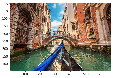
The idea here is to show the power of numpy visually. As images are array, numpy is be used for image transformation. Let’s numpy using this beautiful image of Venice.

from skimage import io
photo = io.imread("venice.jpg")
print("type of image {} . Shape of image {}".format(type(photo), photo.shape) )
import matplotlib.pyplot as plt
plt.imshow(photo)
plt.show()

 

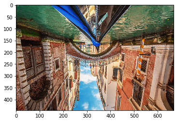
Reverse the image:

plt.imshow(photo[::-1]) ## the row are untouched
## the columns are reversed

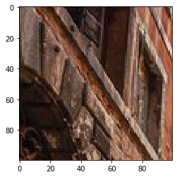
Slice the image using indexes:

plt.imshow(photo[0:100, 100:200])

 

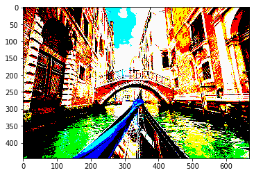
Masked image:

photo_masked = np.where(photo>100, 250, 0)
plt.imshow(photo_masked)

 

Conclusion:

I hope that this tutorial was helpful to rekindle the love for NumPy and will lead to more numpy based functions being implemented. Feel free to comment on NumPy tricks and tips below.

Here is my Linkedin profile in case you want to connect with me. I’ll be happy to be connected with you. Too lazy to type/copy the code? Clone the repo(here).

The media shown in this article are not owned by Analytics Vidhya and are used at the Author’s discretion.

Chrisx10

Data scientist. Extensively using data mining, data processing algorithms, visualization, statistics, and predictive modeling to solve challenging business problems and generate insights. My responsibilities as a Data Scientist include but are not limited to developing analytical models, data cleaning, explorations, feature engineering, feature selection, modeling, building prototype, documentation of an algorithm, and insights for projects such as pricing analytics for a craft retailer, promotion analytics for a fortune 500 wholesale club, inventory management/demand forecasting for a jewelry retailer and collaborating with on-site teams to deliver highly accurate results on time.