Introduction
Does it take you forever to find your lost sock? Do you also find it difficult to search for some particular data on an Excel sheet? While we may not be able to help you with the first, we definitely have an Excel function to help you with the second. Meet the HLOOKUP function! This function, available on both Microsoft Excel and Google Sheets, helps you find specific data values from across a row. You can learn all about the HLOOKUP function, including its implementation in Excel and Google Sheets, with this comprehensive guide. So let’s get started!
Overview
- Understand what the HLOOKUP function in Excel does.
- Know how and where to use the HLOOKUP function in Excel and Google Sheets.
- Learn how to handle the most common errors in using the HLOOKUP function in Excel.

Table of Contents
What is the HLOOKUP Function?
HLOOKUP is short for Horizontal Lookup. It’s a built-in Excel function designed to search for specific values across the top-most row of a table.
Here’s how the function works. It searches for a particular value in the first row of a table or range and returns a corresponding value from a specified row in the same column. This comes in handy when dealing with datasets where the values are arranged horizontally across the top row.
The Syntax of the HLOOKUP function is
=HLOOKUP(lookup_value, table_array, row_index_num, [range_lookup])Let’s break down the components in this formula.
- lookup_value: This is the value you want to search for in the first row of the table or range.
- table_array: This is the range of cells containing the data you want to search. It includes the row with the lookup values and the rows with the corresponding data.
- row_index_num: This is the number of the row in the table_array from which you want to retrieve the value. For example, if you want to get data from the second row, the row_index_num will be 2.
- [range_lookup] (optional): This is a logical value that specifies whether you want an exact match (FALSE) or an approximate match (TRUE). If this argument is omitted, the default is TRUE, which will return an approximate match.
Do check out this Excel article to learn more and further enhance your analytical skills.
Real-Life Example of Applying HLOOKUP
Let us now try to understand the HLOOKUP function better, with a real-life use case. Imagine you are an English teacher who has a spreadsheet with student details. The first row of the sheet contains the names of students and the rows below show their respective test marks. Now, you need to find the test score of a particular student based on their name.
Let’s see how you can do this using the HLOOKUP function in Excel or Google Sheets.
- Set Up the Data
Arrange your data with the names of the student in the first row (e.g., B1:J1) and their corresponding test scores in the rows below (e.g., B2:J6).

- Insert the HLOOKUP Formula
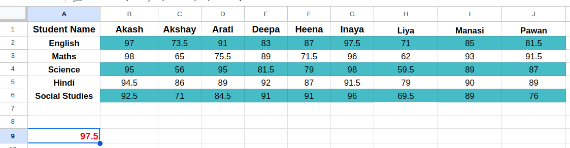
Let’s say you want to find the English test marks of the student named “Inaya” in the sample table created above. For that, you need to enter the following formula into an empty cell:
=HLOOKUP(“Inaya”, A1:J6, 2, FALSE)
Here,
– “Inaya” is the lookup_value you want to search for in the first row (A1:J1).
– A1:J6 is the table_array containing the data.
– 2 is the row_index_num, indicating that you want to retrieve the result from the second row (where the English marks are located). This number would be 3 for Maths, 4 for Science marks, and so on.
– FALSE specifies that you want an exact match for the student’s name.
Once you press Enter, the formula will search for “Inaya” in the first row of the table_array. It will then return the corresponding test score from the second row in the same column.
Here’s the output result:
Possible Errors and How to Fix Them
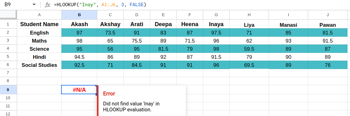
1. #N/A Error: This error occurs when the lookup_value is not found in the first row of the table_array. You can prevent this error by double-checking the spelling and case sensitivity of the lookup_value. Ensure that the table_array includes the lookup_value in its first row.
2. #REF! Error: This error happens when the row_index_num is greater than the number of rows in the table_array. To fix this error, verify that the row_index_num is set correctly and does not exceed the number of rows in the table_array.

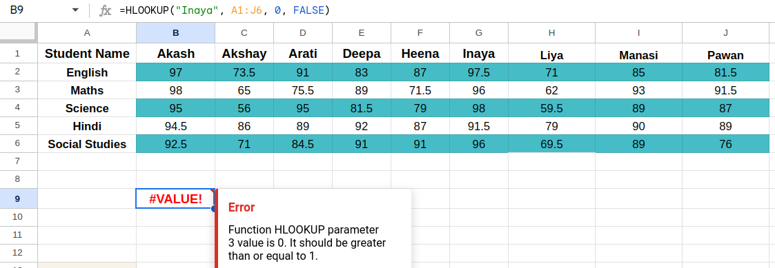
3. #VALUE! Error: This error usually occurs if the row_index_num is less than 1. It can also happen if a non-numeric value is entered by mistake instead of any of the numeric values in the formula. In order to fix this, ensure that the row_index_num is a positive integer, and change any non-numeric values incorrectly put in the formula.
Tips and Best Practices
The following points help you use the HLOOKUP function effectively. They also help you minimize errors and make the most use of the function in your Excel or Google Sheets workflows.
1. Case Sensitivity
The HLOOKUP function is case-insensitive by default. This means it does not differentiate between uppercase and lowercase letters. If at all case sensitivity is important in your data, you can use the EXACT function along with the HLOOKUP function. This way the function performs a case-sensitive lookup.
2. Approximate Match vs. Exact Match
When using [range_lookup] in the HLOOKUP function, you need to decide whether you need an approximate match or an exact match. If your input is TRUE or omitted, if would give an approximate match. If you want an exact match instead, you need to type in FALSE. Also, for an approximate match, the values in the first row of the table_array must be sorted in ascending order.
3. Use of Special Characters
You can also use special characters such as asterisk (*) and question mark (?), for partial matches using the HLOOKUP function. This comes in handy when you need to find values based on partial information.
4. Absolute and Relative Cell References
If you are copying and pasting HLOOKUP formulas, make sure to use absolute cell references ($) for the table_array, to prevent the range from changing. For the lookup_value, you can use relative or mixed cell references depending on your requirements.
5. Error Handling
Did you you can change how the error message is displayed in Excel or Google Sheets? Using the IFERROR function, you can handle errors gracefully and display a custom message instead of an error code. For example, =IFERROR(HLOOKUP(…), “Value not found”) would show that message instead of the error message.
6. Alternative Functions
If the HLOOKUP function does not meet your specific needs, consider using alternative functions. For vertical lookups, you can use VLOOKUP and for more flexibility you can use INDEX/MATCH. The newer XLOOKUP function (introduced in Excel 2019) is also a useful alternative.
7. Test and Validate
It is recommended to first test your HLOOKUP formulas on some sample data and ensure they are working correctly, before applying them to your actual dataset. If you are constantly making changes to the data or formula, then you are also advised to validate the results periodically.
Read more: Advanced Excel for Data Analysis
Conclusion
The HLOOKUP function in Excel and Google Sheets is a great tool to enhance your data analysis and management abilities. Whether you’re a student, a working professional, or simply someone looking to improve their Excel proficiency, understanding how to use HLOOKUP is essential and quite useful. It can help you work more efficiently and make better data-driven decisions. With its ability to search and retrieve data horizontally, HLOOKUP is a powerful tool that should be part of every Excel user’s toolkit.
For further learning, consider exploring this comprehensive course on Microsoft Excel: Formulas & Functions by Analytics Vidhya.
Frequently Asked Questions
Q1. What is HLOOKUP?
A. HLOOKUP (Horizontal Lookup) is a built-in Excel function designed to search for a specific value across the top-most row of a table or a range. It returns a corresponding value from the specified column and is commonly used to fetch data in tables where the data is organized horizontally.
Q2. Can HLOOKUP return values from multiple rows?
A. No, HLOOKUP can only return a value from a single row, specified in the formula. If you wish to find different values from multiple rows, you would need to use the HLOOKUP function multiple times – separately for each row.
Q3. Can HLOOKUP be used with data that isn’t sorted?
A. The HLOOKUP function can be used for an exact match in datasets that are not sorted. However, for an approximate match, the data in the first row of the table_array must be sorted in ascending order.
Q4. How is HLOOKUP different from VLOOKUP?
A. HLOOKUP is used to find specific data values from a table that is horizontally organized, as the function searches horizontally. Meanwhile, VLOOKUP does the same for columns instead of rows, and is used for vertically organized tables.
Sabreena is a GenAI enthusiast and tech editor who's passionate about documenting the latest advancements that shape the world. She's currently exploring the world of AI and Data Science as the Manager of Content & Growth at Analytics Vidhya.


