Kimi K3 Architecture Explained: How a 2.8T Model Runs Efficiently

I started writing this blog when Kimi K3 was still Moonshot’s flagship. Then, on 24th October 2026, Kimi K3.1 Pro dropped, right in the middle of my writing, hehe. The good news: K3.1 Pro is built on the same K3 base model with much more post-training on top, so everything we study here still applies. Moonshot compares it head-to-head with Claude Opus 5.5 and GPT-6 Astra, and on the independent Artificial Analysis index it sits just three points behind Opus 5.5.

K3 itself is worth understanding. It is one of the largest open models, with 2.8T parameters and 896 routed experts, yet it cost over 3x less per token than Claude Fable 5 at list prices. That efficiency comes from a stack of research ideas, including linear attention, mixture of experts and attention residuals, each built to keep costs low without losing quality.

The model is so large that even at 4-bit precision, its weights alone take about 1.4 TB, far more than a single GPU can hold. Its experts are spread across many GPUs, so a single token can hop between several of them before a reply is written.

So how does a model this big run only a fraction of itself for every token? Let’s break it down.

How Big is Kimi K3, and What Might it Take to Run?

Kimi K3 has 2.8 trillion parameters, but only about 104 billion are active for any single token. The catch is that all 2.8 trillion still have to sit in GPU memory, ready to be called.

Even at 4-bit precision, the weights alone take about 1.4 TB. A single NVIDIA Blackwell Ultra GPU (B300) holds 288 GB of memory, so the model needs several GPUs just to load. An 8-GPU DGX B300 node, with about 2.3 TB in total, can fit the weights. That leaves limited room, though, for the context memory (KV cache) and the many requests a production system handles at once.

So at scale, K3’s experts are typically spread across a larger system, such as NVIDIA’s NVL72 rack, which links 72 Blackwell GPUs together. This means a single token may travel across several GPUs to reach the experts it needs. Keep this in mind: much of K3’s design is about making that trip cheaper.

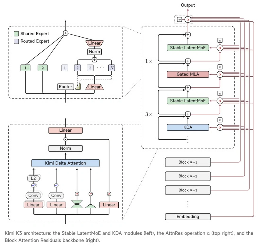
So how does a model this big run only a fraction of itself for every token? Here’s the full architecture at a glance.

Where Kimi K3 Saves Cost: Reading vs. Writing

Inference has two stages. In the reading stage (prefill), the model takes in the whole prompt at once. In the writing stage (decoding), it produces the reply one token at a time. Reading is limited by compute, while writing is limited by memory, because every new token has to pull the weights and the saved context from memory again.

K3 cuts cost in both. Some of its components, though, aren’t about cost at all: they help the model learn better, train stably and handle 1M tokens. Each section below ends with a line on which stage it helps.

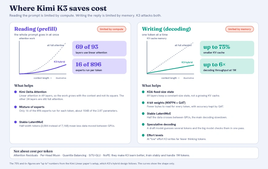
We’ll go through K3 in three parts: how it reads a prompt, how it writes a reply, and how it was trained.

Part 1: How K3 Reads a Prompt

Reading is where K3 takes in your prompt, and with a 1M-token context, that prompt can be enormous. These four ideas decide how K3 processes it, how its layers share what they learn, and how it handles long inputs without slowing to a crawl.

Kimi Delta Attention

Here’s what we are trying to do: make attention cheap enough to handle a 1M-token prompt, without losing the model’s ability to remember what it read. We’ll get there in four steps. Each step fixes a problem left by the one before it.

The Problem: Standard Attention Gets Expensive

When the model reads a prompt (the prefill stage), every token has to be compared with the others in the sequence. That’s the job of attention.

In standard attention, every token directly checks every token before it. This is very expressive, since the model can pull the relevant information from anywhere in the context. But the cost grows quadratically with the context length: double the prompt, and the work roughly quadruples. At 1M tokens, that gets terribly expensive.

That’s why labs look for alternatives. DeepSeek used sparse attention for its V4 model, and Nemotron 3 uses Mamba-2, which replaces most attention layers with a recurrent state-space memory. Kimi K3 builds on a third option: linear attention.

Step 1: Linear Attention, a Fixed-Size Memory

Instead of going back over every previous token, linear attention squeezes the whole sequence into a fixed-size memory called the state. Whenever a new token comes in, the model updates the state, and reads from it for the ongoing context.

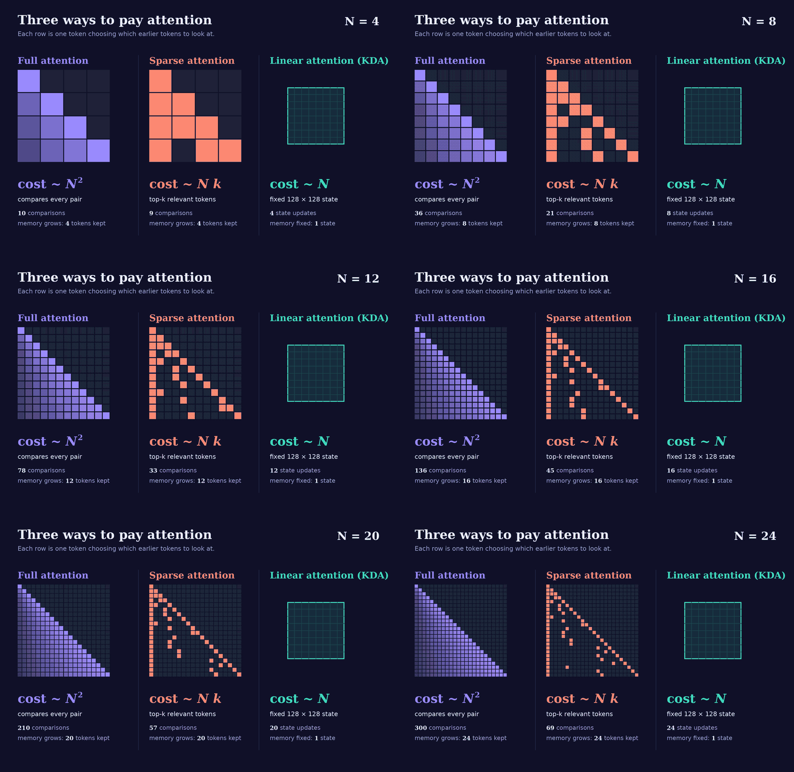
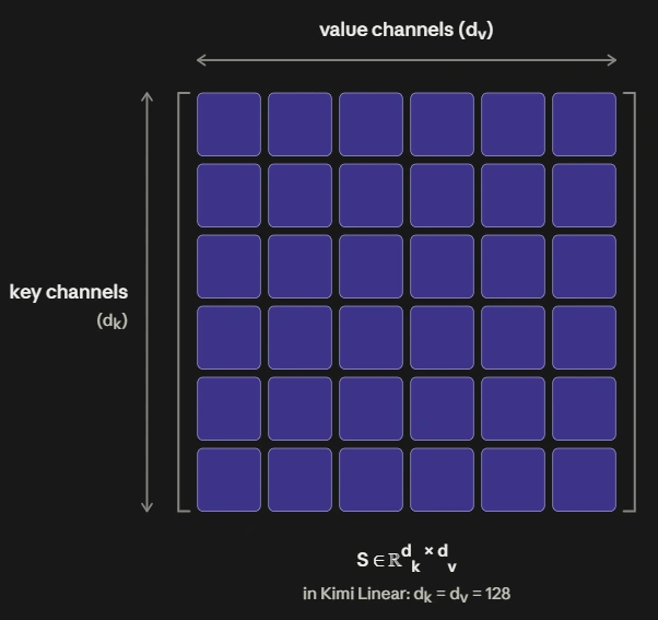
The fixed-size square you see in the GIF is the state. Since it never grows, the memory cost stays fixed no matter how long the context gets. In K3, the state is a 128 × 128 matrix (d_k = d_v = 128). Each row is one key channel, and each column is one value channel. When we say “channel” below, we mean one row of the state.

What’s still broken: squeezing a whole context into a fixed state has historically made linear attention weak. New tokens slowly overwrite old key-value associations, a problem called key-value interference, so information gets lost when the model tries to retrieve it. 🙁

Step 2: The Delta Rule, Only Write What’s New

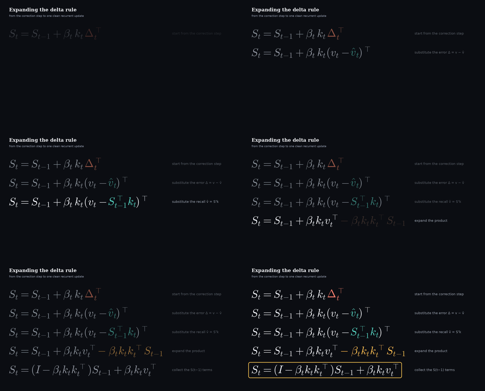
n plain linear attention, every new key-value pair is simply added to the state, without checking what the memory already knows. That blind writing is what causes the interference. The delta rule adds a check first, in three steps:

Step 1: Recall. Ask the memory what it predicts for the current key.
\hat{v}_t = S_{t-1}^{\top} k_t

Step 2: Compare. The gap between that prediction and the real value is the error.
\Delta_t = v_t – \hat{v}_t

Step 3: Correct. Update the memory using only that error.
S_t = S_{t-1} + \beta_t k_t \Delta_t^{\top}

If the memory is already right, the error is zero and nothing changes. That’s where the “Delta” in the name comes from. Combined, the three steps give:

S_t = (I – \beta_t k_t k_t^{\top}) S_{t-1} + \beta_t k_t v_t^{\top}

What’s still broken: old information is never removed, so over time the memory fills up with outdated content.

Step 3: Forgetting, Channel by Channel

The delta rule fixed blind writing, but the memory still has no way to let go. Old information stays in the state forever, even when it’s no longer useful. Over time, the memory fills up with outdated content.

The first fix: a forget gate

Gated DeltaNet, which KDA builds on, adds a forget gate called α, similar to the forget gate in an LSTM. Before each new token is written, the old state is multiplied by α, a number between 0 and 1:

• α close to 1 means “keep almost everything”
• α close to 0 means “forget almost everything”

S_t = \alpha_t (I – \beta_t k_t k_t^{\top}) S_{t-1} + \beta_t k_t v_t^{\top}, \quad \alpha_t \in (0, 1)

The problem: one α for everything

Here, α is a single number applied to the whole state. Every row (channel) forgets at exactly the same speed.

That’s a problem, because different rows hold different kinds of information. One row might hold the topic of a document, which you need for the next 10,000 tokens. Another might hold the last word you read, which is useless a few tokens later. With one α, you can’t keep the first while clearing the second. Either both stay, or both fade.

Think of a whiteboard where you can only erase everything at once, at the same speed. You can’t keep the important notes while wiping the scribbles.

KDA’s fix: one α per channel

KDA gives every row of the state its own α. Mathematically, the single α becomes Diag(α_t):

S_t = (I – \beta_t k_t k_t^{\top}) \mathrm{Diag}(\alpha_t) S_{t-1} + \beta_t k_t v_t^{\top}

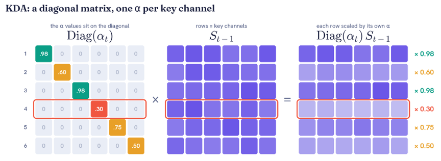
Diag(α_t) is simply a matrix with each row’s α on its diagonal and zeros everywhere else. Multiplying it with the state scales each row by its own α. In the image, row 1 (α = 0.98) barely changes, while row 4 (α = 0.30) fades sharply. Each row now has its own eraser.

These α values aren’t fixed. Every new token passes through a small learned layer that produces a fresh set of α values, one per row. So for every token, two things happen in order:

1. The old state is faded, row by row, using that token’s α values.
2. Then the new information is written in.

What this looks like over time

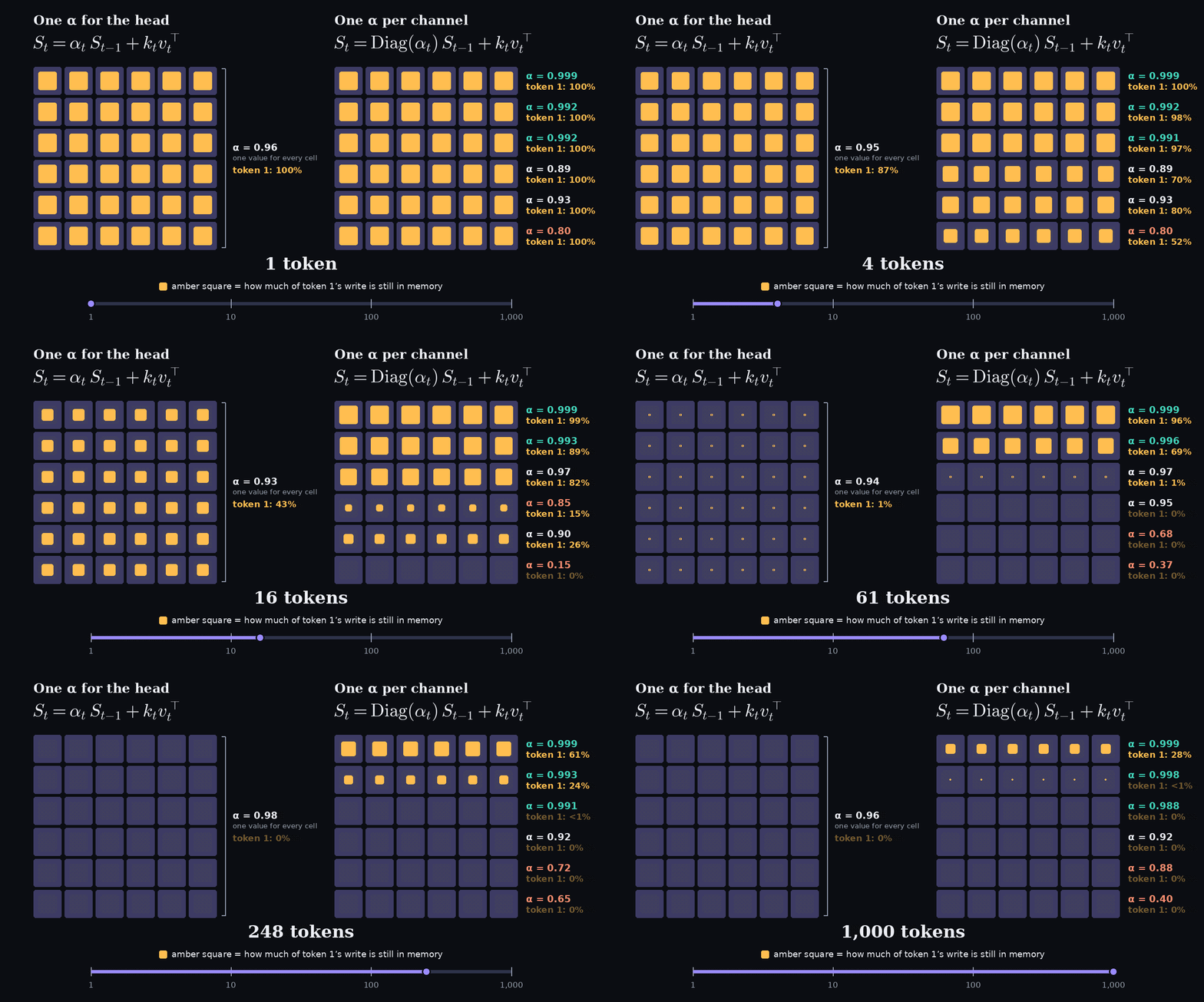
The GIF runs both approaches side by side for 1,000 tokens. Each amber square shows how much of token 1’s information is still in memory.

• Left, one α (Gated DeltaNet): every row fades together. By around 300 tokens, token 1 is completely gone from every row.
• Right, one α per row (KDA): rows with low α clear within a few dozen tokens, but the top row, with α = 0.999, still holds 28% of token 1 after 1,000 tokens.

Same memory size, very different lifespans. Rows with α close to 1 become long-term memory, carrying things like a topic or a name from far back. Rows with lower α become short-term memory, holding recent, local details and clearing them before they go stale.

The GIF shows only the forgetting part of the update, so we can focus on α.

Reading the “token 1: x%” labels

Each label shows how much of token 1’s original write is left in that row. It starts at 100%. After that, every new token multiplies what’s left by that row’s α, so after n tokens, the share is α₂ × α₃ × … × αₙ.

Because it’s a running product, one sharp dip can wipe out most of it at once. That’s why the second row ends at α = 0.998 but holds under 1%: an earlier dip already erased it. (The α values in the GIF are illustrative.)

Here’s the whole journey in one picture:

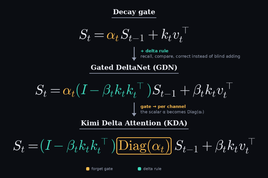
Start with a simple decay gate. Add the delta rule (recall, compare, correct) to get Gated DeltaNet. Then turn the single α into one α per channel to get KDA. This recurrent update is the heart of KDA.

What’s still broken: KDA compresses and organises information far better than plain linear attention, but it’s still a compression. Standard attention wins at exact retrieval, because in a compressed state, the original key-value pairs may no longer exist.

Step 4: The Hybrid Design, Mixing in Full Attention

So K3 doesn’t rely on KDA alone. It interleaves KDA layers with full attention layers in a 3:1 pattern. The full attention layers use Gated MLA (Multi-head Latent Attention), which is full attention with a compressed KV cache. The KDA layers do most of the cheap work, and the full attention layers handle precise retrieval.

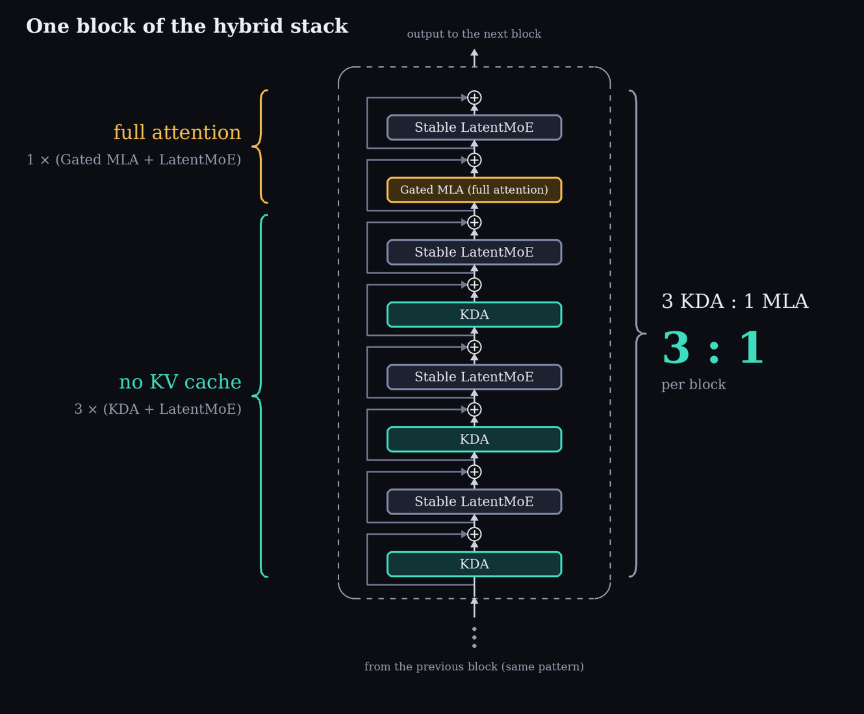
Each block stacks three KDA layers and one Gated MLA layer, each followed by a Stable LatentMoE layer. The three KDA layers keep no KV cache at all.

This ratio, carried over from Moonshot’s Kimi Linear research (October 2025), gave the best balance between quality and speed. Since only about one in four layers stores a KV cache, the cache shrinks by up to 75%, with up to 6x decoding throughput at 1M context.

In the Kimi Linear paper, Moonshot tested this design on a 48B-parameter MoE with 3B active parameters, trained on 1.4T tokens alongside a full attention baseline (MLA) and a Gated DeltaNet hybrid (GDN-H), for a fair comparison.

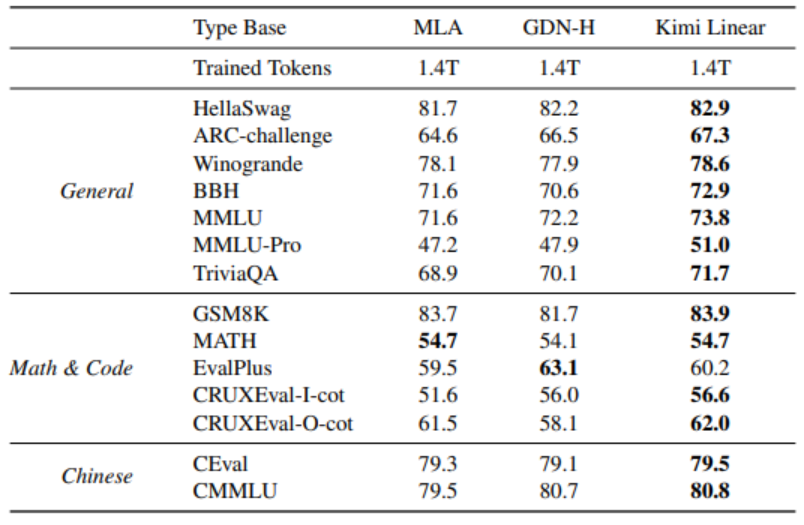
Kimi Linear matched or beat full attention on most benchmarks, including MMLU-Pro (51.0 vs 47.2). It also held up on the 128K-context RULER benchmark, and at 1M tokens, its time per output token dropped from 11.48 ms to 1.84 ms.

Kimi Linear paper: https://arxiv.org/pdf/2510.26692

Inside a KDA Layer

Now let’s see how all four steps come together in one layer.

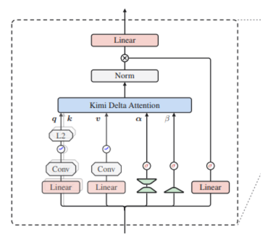
The layer’s input splits into parallel branches. The q, k and v branches each pass through a linear layer, a short convolution and an activation. q and k are also scaled to length 1. This keeps the memory stable: at every token, the old state is multiplied by (I − β k kᵀ), and a key of length 1 guarantees that this step can only keep or shrink the state, never blow it up.

Two more branches control the memory itself:

• α, the forget gate, has a lot to produce: one decay value for every channel, for every token, in every head. A full linear layer for that would be expensive, so a low-rank projection (the hourglass shape) squeezes the input down and expands it back out, which is much cheaper. A sigmoid then keeps each value between 0 (forget) and 1 (remember), so α can only keep or shrink the memory, never amplify it.
• β, the write strength, needs only one number per head, so a single small projection is enough (the single triangle). Its sigmoid keeps β between 0, meaning skip this token, and 1, meaning fully overwrite what the key points to.

All of these feed into the KDA box, where the state is decayed, corrected and read out using the formula we just built. The result is normalised, multiplied element-wise (⊗) by an output gate that decides how much passes through, and sent through a final linear layer.

This is how KDA improves both phases. In reading, 69 of K3’s 93 layers process the prompt with linear attention, so their cost grows linearly with the context. The 24 full attention layers still grow quadratically, which is why this is a big saving but not a cure. In writing, those same KDA layers keep a fixed-size state instead of a growing KV cache, which cuts the cache by up to 75% and gives up to 6x decoding throughput at 1M context.

Attention Residuals

Here’s what we are trying to do: help information travel cleanly through all 93 of K3’s layers, so deep layers can still use what early layers learned.

Most of us have heard of residual connections. ResNet introduced them during the ImageNet competition, and they changed how deep networks are built. Each layer’s output is added to a running sum, so the original information isn’t lost as the network gets deeper.

The problem with standard residuals: every earlier layer’s output is added with the same weight of 1. As the model gets deeper, the running sum keeps growing, and each layer’s own contribution gets diluted. A layer can’t choose which earlier layers matter for the token it’s processing.

The fix: attention residuals let each layer use softmax attention over the outputs of the earlier layers. Each layer gets its own learned query, which scores every earlier output, the embedding included. The scores become weights that sum to 1, so the layer can lean on whichever earlier representations are actually useful.

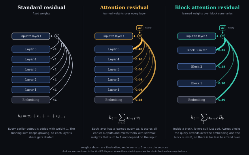
The left panel is a standard residual, where every earlier output is added with the same weight. The middle panel is the attention residual, where each layer weighs all the earlier outputs, and a thicker line means more weight. The right panel is the block version.

Why K3 uses blocks: attending over all 93 layers individually would be costly. So inside a block, layers still just add. Across blocks, each layer’s query attends over the embedding and a few block summaries.

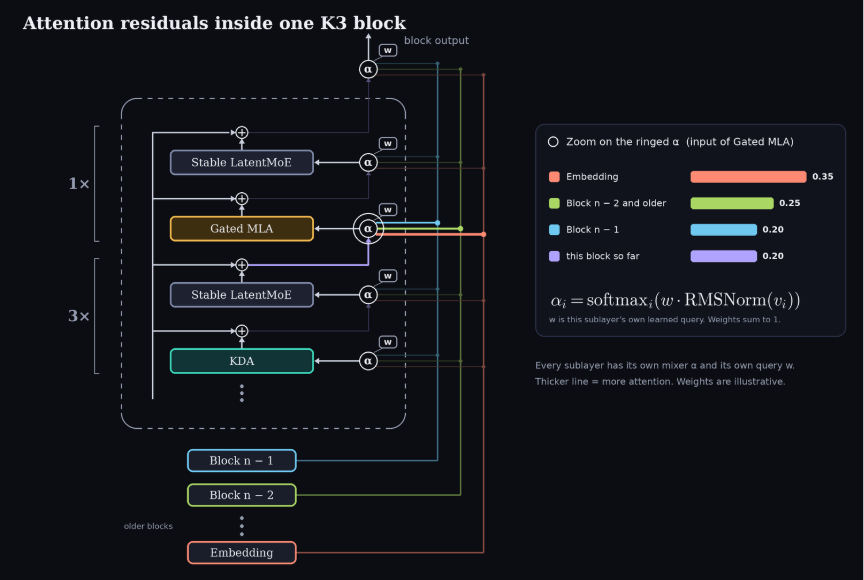
Every sublayer has its own small mixer with its own learned query. The mixer blends the embedding, the earlier blocks and the current block so far. The zoom box shows the weights chosen by one mixer: here, the input to Gated MLA draws 35% from the embedding, 25% from older blocks, and 20% each from the previous block and the current one.

The key idea is that attention now works across layers, not just across tokens. Instead of one fixed running sum, every sublayer chooses what to read from the layers below it, which gives the model stronger learning dynamics.

This is how Attention Residuals fit in. They don’t make reading or writing cheaper. They improve how well the model learns and uses its earlier layers, so think of them as a quality upgrade, not a speed-up. Inference engines use a fused kernel to keep their small extra cost down.

Stable LatentMoE

Here’s what we are trying to do: run a 2.8T-parameter model while only using a small slice of it per token, and keep the traffic between GPUs from slowing everything down.

Remember the size problem from the start? K3’s experts are scattered across many GPUs, which talk to each other over interconnects like NVLink and NVSwitch.

K3 is a Mixture of Experts (MoE) with 896 routed experts, 2.3x the 384 experts in Kimi K2. But only 16 experts run for each token, an activation rate of just 1.8%. Compare that with MiniMax M3 at 3.1%, Nemotron 3 Ultra at 4.3% and Kimi K2 at 2%. So out of 2.8T parameters, only about 104B are active per token. You get a giant model’s knowledge at a fraction of the running cost.

The problem: in a normal MoE, each token sends its complete hidden state to whichever GPU hosts its expert. With this many experts spread across this many GPUs, moving that data becomes slow and expensive.

The fix, LatentMoE: compress the token before sending it to the experts, then expand it back afterwards. Less data crosses between GPUs, so processing gets faster.

Why “Stable”? Very sparse MoEs are hard to train. The router can keep sending tokens to the same few popular experts, which overloads them and leaves the rest idle and untrained. In the worst case, training collapses. Activations can also blow up in a model this large. “Stable” refers to the three pieces that keep training steady: Quantile Balancing, SiTU-GLU and an RMSNorm, all covered below.

How Stable LatentMoE Works?

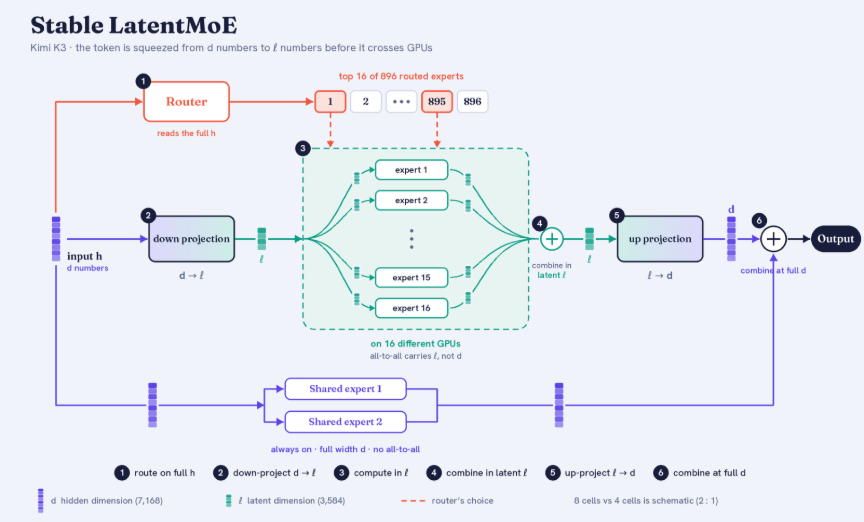
Follow the six numbered steps in the image:

1. Route on the full h. The token arrives as a vector of 7,168 numbers. The router reads all of it and picks the top 16 of the 896 routed experts. Routing happens before any compression, so the choice uses full information.
2. Down-project d → ℓ. A learned projection squeezes the token from 7,168 numbers to 3,584, half the size.
3. Compute in ℓ. The half-width token goes to the 16 chosen experts on different GPUs. The traffic between GPUs now carries half the data per token. This is where the saving comes from.
4. Combine in latent ℓ. The 16 expert outputs come back, still half-width, and are mixed into one vector.
5. Up-project ℓ → d. One projection takes the mixed vector back to full width.
6. Combine at full d. The result is added to the output of the two shared experts, which are always on. They run at full width and never send anything across GPUs.

Here’s what that saving looks like in practice:

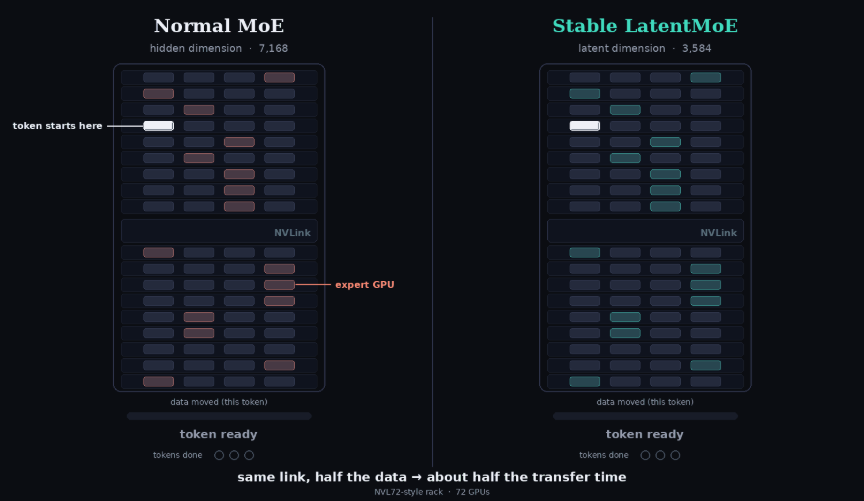
Both sides show the same NVL72-style rack of 72 GPUs, with a token travelling over NVLink to its expert GPUs. On the left, a normal MoE sends the full 7,168-number token. On the right, Stable LatentMoE sends the 3,584-number version. Same link, half the data, so about half the transfer time. Fewer numbers per token also means less compute inside each expert.

Note that the “Stable” parts are about training, so they aren’t shown here. We’ll cover them next.

Quantile Balancing

With 896 experts and only 16 active per token, the router can easily fall into a rut. If it keeps favouring the same experts, the others stay undertrained and the model loses part of its capacity.

The popular fix, used in DeepSeek-V3, adds a bias to each expert’s score and nudges it by a fixed step whenever the expert is over- or underloaded. Across nearly a thousand experts, that step-by-step nudging is slow and hard to tune.

K3 keeps the bias but calculates it directly. Each expert should get its fair share of tokens, 16/896, or about 1 in 56. Quantile Balancing sets each expert’s bias so it wins exactly that share. Think of it as grading on a curve: instead of one fixed pass mark, each expert gets the cutoff that admits exactly its fair share.

How the router picks experts

For every token, the router gives each of the 896 experts a score, and the token goes to the 16 with the best scores. With raw scores alone, the same favourites win again and again.

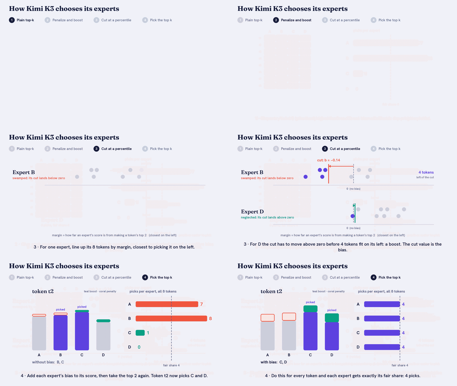
The GIF uses a tiny example: 8 tokens, 4 experts, and 2 picks per token. The fair share is 4 picks each (8 × 2 ÷ 4).

In step 1 (Plain top-k), each token simply takes its 2 highest scores. The counts come out uneven: A gets 7, B gets 8, C gets 1 and D gets 0.

In step 2 (Penalize and boost), each expert gets a bias added to its score, only when choosing the top experts. Overpicked experts get a negative bias (a penalty), and underpicked experts get a positive bias (a boost). A and B’s bars go left of zero, and C and D’s go right.

How each bias is set

For each expert, K3 does four things:

1. Measure the margin. For every token, check how far the expert was from making the top picks. It’s negative if the expert made the cut, positive if it missed.
2. Line the tokens up, from the smallest margin (where the expert did best) to the largest.
3. Find the fair share: 4 tokens in the toy, about 1 in 56 in K3.
4. Cut the line there. The margin at the cut is the bias.

A quick example: an expert wins 6 tokens but should only win 3. Its wins were by 8, 6, 5, 3, 2 and 1 points. Its third-biggest win was by 5 points, so K3 takes 5 points off its score. Now only its 3 strongest wins survive. That “minus 5” is its bias.

It works in reverse too. If an expert’s three closest misses were by 2, 4 and 5 points, K3 adds 5 points, and it now wins those 3 tokens.

In step 3 of the GIF (Cut at a percentile), each dot is a token, sorted by margin. Purple dots are tokens the expert wins, and grey dots are ones it loses. A cut line slides from zero until exactly 4 purple dots sit on its left:

• Expert B was swamped, so the line slides left about 0.14. Its bias is −0.14, a penalty.
• Expert D was barely picked, so the line slides right about 0.15. Its bias is +0.15, a boost.

(B starts with 5 dots on its left, not 8, because step 3 shows each expert with the other experts’ biases already applied. The real router sets all the biases together.)

In step 4 (Pick the top k), the biases are added and each token picks again. Token t2’s raw scores point to B and C, but after the biases, it picks C and D. Across all tokens, the counts even out to 4 each.

Two practical details:

• An exact quantile over millions of tokens across GPUs isn’t feasible, so each expert keeps a histogram. One all-reduce of integer counters per step is enough to recover the quantile.
• The bias only decides which experts get picked. It doesn’t change how much each chosen expert counts. Those weights still come from the original scores, and balancing targets the whole global batch, not each sentence.

SiTU-GLU

The problem: activation explosion. Each expert sends the token down two parallel branches, a gate branch and a value branch, and multiplies the results. This is a gated linear unit (GLU). K2 used SwiGLU for this. But multiplying large numbers makes them larger, and K3’s routed path chains several matrix multiplications. At 2.8T parameters, activations can blow up.

The fix: SiTU-GLU (Sigmoid Tanh Unit GLU) gives each branch a soft ceiling using a tanh curve. The gate is capped at 4 and the value at 25, so an expert’s output can never exceed 4 × 25 = 100:

\text{SiTU-GLU}(x) = \left[ 4 \cdot \tanh(W_g x / 4) \odot \sigma(W_g x) \right] \odot \left[ 25 \cdot \tanh(W_u x / 25) \right]

For normal values, it behaves like SwiGLU. With inputs of 1 and 1, SwiGLU gives 0.73 and SiTU-GLU gives 0.72. With extreme inputs (50 and 200), SwiGLU gives 10,000, while SiTU-GLU gives 100. Because the ceiling is a smooth curve, not a hard cutoff, gradients still flow during training.

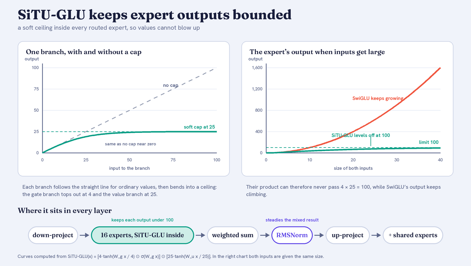
The left chart shows one branch: it follows a straight line for ordinary values, then bends into a ceiling. The right chart shows the expert’s output as inputs grow: SwiGLU keeps climbing, while SiTU-GLU levels off at 100. The strip at the bottom shows where it sits in every layer.

The full routed path runs: down-project, the 16 chosen experts, a weighted sum, an RMSNorm, then up-project, before adding the shared experts. SiTU-GLU keeps each expert’s output bounded, and the RMSNorm steadies the mixed result, whose scale would otherwise vary with which experts were chosen.

Quantile Balancing, SiTU-GLU and the RMSNorm are the three pieces that keep K3’s training stable at 896 experts.

This is how Stable LatentMoE improves both phases. Only 16 of 896 experts run per token, so reading needs far less compute and writing fetches far fewer weights. The half-width tokens cut GPU-to-GPU traffic, which matters most in writing, where that traffic is the main slowdown. SiTU-GLU and Quantile Balancing don’t change speed directly, but balanced experts also mean fewer idle GPUs when serving.

NoPE (No Explicit Positional Encoding)

Here’s what we are trying to do: let K3 handle 1M tokens without patching how it tracks word order.

Attention on its own doesn’t know the order of tokens. A model needs some way to know that one word came before another, which is the job of positional encoding.

The common approach, RoPE: rotary position embedding rotates each query and key by an angle based on the token’s position, so attention scores depend on how far apart two tokens are. It works well, but when you want a longer context than the model trained on, the rotations meet angles they’ve never seen. Teams then have to rescale or stretch the rotation frequencies.

K3’s approach, NoPE: no positional encoding at all in its full attention (MLA) layers. K3 gets its sense of order from KDA instead. KDA reads tokens in order and decays old information with α, so its state naturally carries a sense of how long ago things happened.

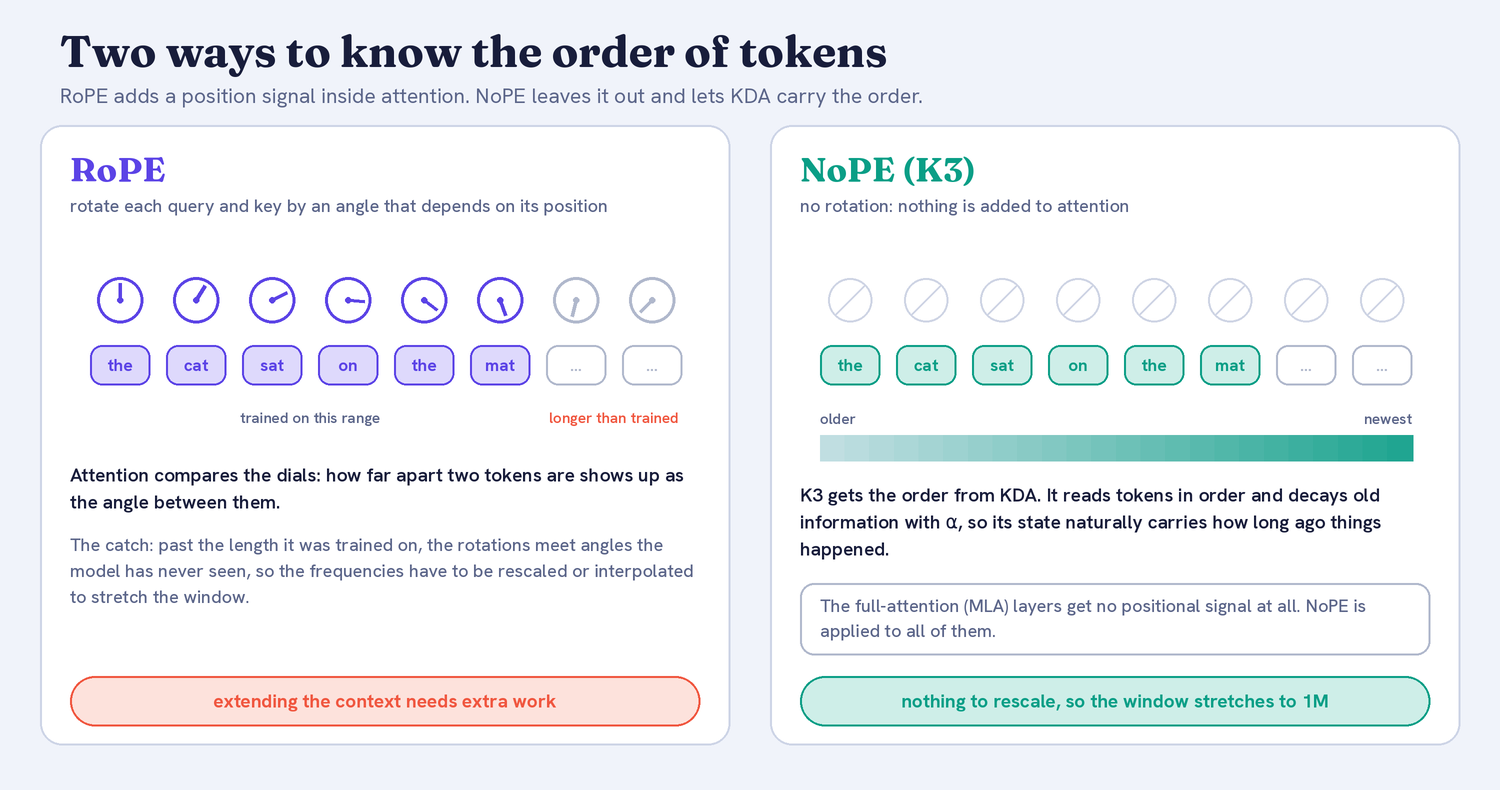
On the left, RoPE gives each token a dial, and past the trained range, the dials point at angles the model has never seen. On the right, NoPE adds nothing, and the order comes from KDA’s fading memory, from older to newest.

With no rotation frequencies, there’s nothing to rescale, and the model extends to 1M tokens without any positional-encoding changes.

This is how NoPE fits in. It doesn’t make either phase cheaper per token. It’s what lets K3 take in a 1M-token prompt cleanly, so it supports the reading phase at very long context.

Part 2: How K3 Writes a Reply

So far we’ve seen how K3 reads a prompt. Now let’s see how it writes the reply.

Writing means producing tokens one by one. For every new token, the GPU has to fetch the weights it needs from memory, about 104 billion active weights in K3’s case, and then repeat the trip for the next token.

Think of a chef (the GPU’s compute cores) who has to walk to a warehouse (memory) to fetch ingredients (weights) for every dish (every token). The cooking is fast. The walk is the slow part. There are three ways to speed things up:

• Pack ingredients into smaller parcels, so each trip carries less (4-bit weights)
• Fetch only what the dish needs (only 16 of 896 experts run, covered in Part 1)
• Cook several dishes per trip (speculative decoding)

4-bit Quantization (MXFP4)

Here’s what we are trying to do: shrink every weight so each trip to memory carries less.

At 16 bits per value, 2.8 trillion weights would take about 5.6 TB, which is very hard to deploy. At 4 bits, that drops to about 1.4 TB.

K3 uses a format called MXFP4, which OpenAI also uses for some of its models. “MX” stands for microscaling: each value takes only 4 bits, but small groups of values share one scale factor, so the group can still cover a useful range of numbers. K3 uses MXFP4 for its expert weights, which make up most of the model, and MXFP8 (the 8-bit version) for activations, the numbers flowing between layers.

This is how 4-bit weights improve the writing phase. Decoding is limited by how fast weights can be read from memory, so 4-bit weights mean fewer bytes per token. They help reading less, since reading is limited by compute.

Quantization-Aware Training (QAT)

Here’s what we are trying to do: shrink the model to 4 bits without losing accuracy.

Compressing a model usually costs accuracy. The common approach is to train in full precision and squeeze to 4 bits at the end. The model never gets a chance to adapt, so some of what it learned is lost in the rounding.

K3 trains while already using the compressed numbers, so it learns to stay accurate despite the rounding. It’s like a student who practises with rounded numbers from the start, instead of working with exact numbers and rounding only the final answer.

QAT starts at supervised fine-tuning (SFT) and continues through reinforcement learning. The same 4-bit scheme is used in training and serving, so what the model practises on is exactly what gets deployed. Pre-training itself isn’t described as 4-bit.

This is how QAT fits in. It doesn’t speed anything up by itself. It makes the 4-bit speed-up usable, by keeping the model accurate after compression.

Speculative Decoding (EAGLE-3)

Here’s what we are trying to do: produce several tokens per pass instead of one.

Normally, the big model produces one token per pass. With speculative decoding, a small draft model quickly guesses the next few tokens, and the big model checks them all in a single pass. Correct guesses are kept, and everything after the first wrong guess is thrown away. This is the “cook several dishes per trip” idea.

If you want a deeper dive, read my earlier blog on speculative decoding.

K3 was designed for this from the start. It’s pre-trained with an extra layer that predicts upcoming tokens, called multi-token prediction (MTP). Later, that layer is fine-tuned into an EAGLE-3-style draft model, with the main model frozen, and trained to maximise how often its guesses are accepted. During training, the draft runs seven steps ahead, feeding on its own earlier guesses, just as it does when serving.

This is how speculative decoding improves the writing phase. During decoding, the compute cores sit idle waiting on memory. The draft model puts that idle compute to work, so each pass produces several tokens. It doesn’t help reading, which already processes many tokens at once.

Part 3: How K3 is Trained

Now let’s look at how K3 learned: the optimizer, the long-context curriculum and the distillation step.

Per-Head Muon

Here’s what we are trying to do: make sure every part of the model learns at a fair pace.

An optimizer decides how every weight changes after each learning step. K3 uses Muon, as K2 did.

The idea behind Muon: the update a model wants to make is usually dominated by a few strong directions, meaning combinations of weights that move together. Those loud directions soak up most of the learning, while the quiet ones barely move. Muon rebalances the update so every direction gets a similar-sized step. It’s like a teacher making sure every student gets a turn to speak.

Why per-head: an attention layer has many heads, each looking at the sequence its own way. If the update is applied to whole attention matrices, a few heads with large gradients can dominate. Per-Head Muon splits the Q, K and V updates by head and balances each head’s update separately, so learning is even across heads.

This mirrors Quantile Balancing. One evens out the work across experts, the other evens out learning across update directions. Both stop a few dominant parts from taking over.

This is how Per-Head Muon fits in. It’s a training technique, so it doesn’t change the cost of reading or writing. It helps the model learn more evenly across its attention heads.

Training for 1M Tokens

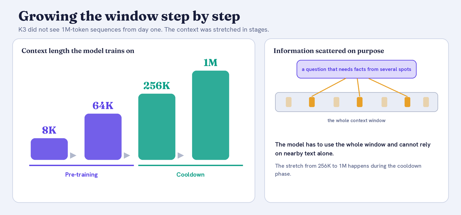
K3 didn’t train on 1M-token sequences from day one. The context window grew in stages: from 8K to 64K tokens during pre-training, then from 256K to 1M during the cooldown phase.

The training also included synthetic tasks where the information needed for the answer was deliberately scattered across the whole context. That forces the model to use the entire window instead of relying on nearby text.

Distillation

Here’s what we are trying to do: get the strengths of many specialist models into one.

K3’s post-training uses multi-teacher on-policy distillation. First, the team trained nine specialist models with reinforcement learning, one for each combination of three domains (general, general agents and coding) and three reasoning-effort levels (low, high and max). Then all nine were merged into a single model.

On-policy means the student learns from its own attempts. It generates an answer, and the teacher matching that task’s domain and effort level grades it token by token. Because the feedback is on the student’s current attempts, not on fixed answers written earlier, it targets the mistakes the student is actually making.

Why not just keep nine models? Each would be a 2.8T-parameter model. You’d need enough GPUs to host all nine, plus a system to route every request to the right one. Distillation teaches one model all nine behaviours instead.

The effort level is simply how long the model thinks before answering. At “low,” it thinks briefly and replies quickly. At “max,” it can spend a minute or more on a hard problem. In K3’s API, you choose it with the reasoning_effort setting: “low”, “high” or “max”, with max as the default. The domain doesn’t need a setting, since it’s picked up from the prompt. It’s like one car with three driving modes instead of nine cars.

This is how distillation helps the writing phase. It doesn’t change the cost per token, but the effort levels let you control how long K3 thinks. At “low” effort, it writes far fewer thinking tokens, so replies are cheaper and faster.

Conclusion

Kimi K3 is a stack of smaller ideas, each aimed at a specific cost. When reading, Kimi Delta Attention keeps most layers linear, and only 16 of 896 experts run per token. When writing, the small KDA state shrinks the KV cache by up to 75%, 4-bit weights cut what each token reads from memory, Stable LatentMoE halves GPU-to-GPU traffic, and speculative decoding produces several tokens per pass. The rest, Attention Residuals, Per-Head Muon, Quantile Balancing, SiTU-GLU and NoPE, help the model learn better, train stably and handle 1M tokens.

Kimi K3.1 Pro builds on this same architecture, with far more post-training on top. Moonshot reports it reaches 65.7% on Terminal-Bench 4.0, just behind Claude Opus 5.5’s 66.4%, and cuts its hallucination rate on a factual stress test from 23.4% to 8.3%. With full open weights promised by 4 November, the architecture behind it is about to become something anyone can study and run.