Overview
- SQL is a must-know language for anyone in analytics or data science
- Here are 8 nifty SQL techniques for data analysis that ever analytics and data science professional will love working with
Introduction
SQL is a key cog in a data science professional’s armory. I’m speaking from experience – you simply cannot expect to carve out a successful career in either analytics or data science if you haven’t yet picked up SQL.
And why is SQL so important?
As we move into a new decade, the rate at which we are producing and consuming data is skyrocketing by the day. To make smart decisions based on data, organizations around the world are hiring data professionals like business analysts and data scientists to mine and unearth insights from the vast treasure trove of data.
And one of the most important tools required for this is – you guessed it – SQL!

Structured Query Language (SQL) has been around for decades. It is a programming language used for managing the data held in relational databases. SQL is used all around the world by a majority of big companies. A data analyst can use SQL to access, read, manipulate, and analyze the data stored in a database and generate useful insights to drive an informed decision-making process.
In this article, I will be discussing 8 SQL techniques/queries that will make you ready for any advanced data analysis problems. Do keep in mind that this article assumes a very basic knowledge of SQL.
I would suggest checking out the below courses if you’re new to SQL and/or business analytics:
Table of Contents
- Let’s First Understand the Dataset
- SQL Technique #1: Counting Rows and Items
- SQL Technique #2: Aggregation Functions
- SQL Technique #3: Extreme Value Identification
- SQL Technique #4: Slicing Data
- SQL Technique #5: Limiting Data
- SQL Technique #6: Sorting Data
- SQL Technique #7: Filtering Patterns
- SQL Technique #8: Groupings, Rolling up Data and Filtering in Groups
Let’s First Understand the Dataset
What is the best way to learn data analysis? By performing it side by side on a dataset! For this purpose, I have created a dummy dataset of a retail store. The customer data table is represented by ConsumerDetails.
Our dataset consists of the following columns:
- Name – The name of the consumer
- Locality – The locality of the customer
- Total_amt_spend – The total amount of money spent by the consumer in the store
- Industry – It signifies the industry from which the consumer belongs to
Note:- I will be using MySQL 5.7 for going forward in the article. You can download it from here – My SQL 5.7 Downloads.

SQL Technique #1 – Counting Rows and Items
-
Count Function
We will begin our analysis with the simplest query, i.e, counting the number of rows in our table. We will do this by using the function – COUNT().

Great! Now we know the number of rows in our table which is 10. It may seem to be funny using this function on a small test dataset but it can help a lot when your rows run into the millions!
-
Distinct Function
A lot of times, our data table is filled with duplicate values. To attain the unique value, we use the DISTINCT function.
In our dataset, how can we find the unique industries that customers belong to?
You guessed it right. We can do this by using the DISTINCT function.

You can even count the number of unique rows by using the count along with distinct. You can refer to the below query:

SQL Technique #2 – Aggregation Functions
Aggregation functions are the base of any kind of data analysis. They provide us with an overview of the dataset. Some of the functions we will be discussing are – SUM(), AVG(), and STDDEV().
-
Calculate sum
We use the SUM() function to calculate the sum of the numerical column in a table.
Let’s find out the sum of the amount spent by each of the customers:

In the above example, sum_all is the variable in which the value of the sum is stored. The sum of the amount of money spent by consumers is Rs. 12,560.
-
Calculate the average
To calculate the average of the numeric columns, we use the AVG() function. Let’s find the average expenditure by the consumers for our retail store:

The average amount spent by customers in the retail store is Rs. 1256.
-
Calculate standard deviation
If you have looked at the dataset and then the average value of expenditure by the consumers, you’ll have noticed there’s something missing. The average does not quite provide the complete picture so let’s find another important metric – Standard Deviation. The function is STDDEV().

The standard deviation comes out to be 829.7 which means there is a high disparity between the expenditures of consumers!
SQL Technique #3 – Extreme Value Identification
The next type of analysis is to identify the extreme values which will help you understand the data better.
-
Max
The maximum numeric value can be identified by using the MAX() function. Let’s see how to apply it:

The maximum amount of money spent by the consumer in the retail store is Rs. 3000.
-
Min
Similar to the max function, we have the MIN() function to identify the minimum numeric value in a given column:

The minimum amount of money spent by the retail store consumer is Rs. 350.
SQL Technique #4 – Slicing Data
Now, let us focus on one of the most important parts of the data analysis – slicing the data. This section of the analysis is going to form the basis for advanced queries and help you retrieve data based on some kind of condition.
- Let’s say that the retail store wants to find the customers coming from a locality, specifically Shakti Nagar and Shanti Vihar. What will be the query for this?

Great, we have 3 customers! We have used the WHERE clause to filter out the data based on the condition that consumers should be living in the locality – Shakti Nagar and Shanti Vihar. I didn’t use the OR condition here. Instead, I have used the IN operator which allows us to specify multiple values in the WHERE clause.
- We need to find the customers who live in specific localities (Shakti Nagar and Shanti Vihar) and spend an amount greater than Rs. 2000.

In our dataset, only Shantanu and Natasha fulfill these conditions. As both conditions need to be fulfilled, the AND condition is better suited here. Let’s check out another example to slice our data.
- This time the retail store wants to retrieve all the consumers who are spending between Rs. 1000 and Rs. 2000 so as to push out special marketing offers. What will be the query for this?

Another way to write the same statement would be:

Only Rohan is clearing this criteria!
Great! We have reached halfway in our journey. Let us build more on the knowledge that we have gained so far.
SQL Technique #5 – Limiting Data
-
Limit
Let’s say we want to view the data table consisting of millions of records. We can’t use the SELECT statement directly as this would dump the complete table onto our screen which is cumbersome and computationally intensive. Instead, we can use the LIMIT clause:

The above SQL command helps us show the first 5 rows of the table.
-
OFFSET
What will you do if you just want to select only the fourth and fifth rows? We will make use of the OFFSET clause. The OFFSET clause will skip the specified number of rows. Let’s see how it works:

SQL Technique #6 – Sorting Data
Sorting data helps us put our data into perspective. We can perform the sorting process by using the keyword – ORDER BY.
-
ORDER BY
The keyword can be used to sort the data into ascending or descending order. The ORDER BY keyword sorts the data in ascending order by default.
Let us see an example where we sort the data according to the column Total_amt_spend in ascending order:

Awesome! To order the dataset into descending order, we can follow the below command:

SQL Technique #7 – Filtering Patterns
In the earlier sections, we learned how to filter the data based on one or multiple conditions. Here, we will learn to filter the columns that match a specified pattern. To move forward with this, we will first understand the LIKE operator and wildcard characters.
-
LIKE operator
The LIKE operator is used in a WHERE clause to search for a specified pattern in a column.
-
Wildcard Characters
The Wildcard Character is used to substitute one or more characters in a string. These are used along with the LIKE operator. The two most common wildcard characters are:
-
- % – It represents 0 or more number of characters
- _ – It represents a single character
In our dummy retail dataset, let’s say we want all the localities that end with “Nagar”. Take a moment to understand the problem statement and think about how we can solve this.
Let’s try to break down the problem. We require all the localities that end with “Nagar” and can have any number of characters before this particular string. Therefore, we can make use of the “%” wildcard before “Nagar”:

Awesome, we have 6 localities ending with this name. Notice that we are using the LIKE operator to perform pattern matching.
Next, we will try to solve another pattern-based problem. We want the names of the consumers whose second character has “a” in their respective names. Again, I would suggest you to take a moment to understand the problem and think of a logic to solve it.
Let’s breakdown the problem. Here, the second character needs to be “a”. The first character can be anything so we substitute this letter with the wildcard “_”. After the second character, there can be any number of characters so we substitute those characters with the wildcard “%”. The final pattern matching will look like this:

We have 6 people satisfying this bizarre condition!
SQL Technique #8 – Groupings, Rolling up Data and Filtering in Groups
We have finally arrived at one of the most powerful analysis tools in SQL – Grouping of data which is performed using the GROUP BY statement. The most useful application of this statement is to find the distribution of categorical variables. This is done by using the GROUP BY statement along with aggregation functions like – COUNT, SUM, AVG, etc.
Let’s try to understand this better by taking up a problem statement. The retail store wants to find the Number of Customers corresponding to the industries they belong to:

We notice that the count of customers belonging to the various industries is more or less the same. So, let us move forward and find the sum of spendings by customers grouped by the industry they belong to:

We can observe that the maximum amount of money spent is by the customers belonging to the Manufacturing industry. This seems a bit easy, right? Let us take a step ahead and make it more complicated.
Now, the retailer wants to find the industries whose total_sum is greater than 2500. To solve this problem, we will again group by the data according to the industry and then use the HAVING clause.
-
HAVING
The HAVING clause is just like the WHERE clause but only for filtering the grouped by data. Remember, it will always come after the GROUP BY statement.
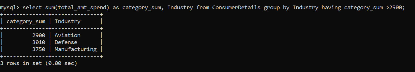
We have only 3 categories that satisfy the conditions – Aviation, Defense, and Manufacturing. But to make it more clearer, I will also add the ORDER BY keyword to make it more intuitive:

End Notes
I am really glad you made it so far. These are the building blocks for all data analysis queries in SQL. You can also take up advanced queries by using these fundamentals. In this article, I made use of MySQL 5.7 to establish the examples.
I really hope that these SQL queries will help you in your day to day life when you are analyzing complex data. Do you have any of your tips and tricks for analyzing data in SQL? Let me know in the comments!
Product Growth Analyst at Analytics Vidhya. I'm always curious to deep dive into data, process it, polish it so as to create value. My interest lies in the field of marketing analytics.


Best and knowledge full blog 💓💓💓, Thanks a lot
The article was really helpful to me . I've also learned some new queries and found it useful in my daily routine . Thanks to all VIDHYA ANALYTICS for providing good articles and various courses.
Good , simple n short article