This article was published as a part of the Data Science Blogathon
Introduction
This article is part of an ongoing blog series on Natural Language Processing (NLP). In the previous article, we discussed a Topic modelling technique named Latent Semantic Analysis (LSA), but we observed that there are some disadvantages of LSA, so to overcome those problems, we come up with the concept of pLSA, which stands for Probabilistic Latent Semantic Analysis.
So, In this article, we will deep dive into the concepts of pLSA, which is a technique used to model information under a probabilistic framework, and also discuss the mathematics behind the different parametrization of this technique in a detailed manner.
This is part-17 of the blog series on the Step by Step Guide to Natural Language Processing.
Table of Contents
1. Familiar with variables involved in pLSA
2. What is pLSA?
3. Latent Variable Model for pLSA
4. Matrix Factorization model for pLSA
5. Advantages and Disadvantages of pLSA
Familiar with Variables involved in pLSA
We have to understand the following three sets of variables while studying pLSA:
- Documents
- Words
- Topics
Let’s discuss each of them one by one in a bit detailed manner:
Documents
Representation: D={d1,d2,d3,…dN}
where N represents the number of documents present in the corpus.
di denotes ith document in the set D.
Here we can call a document also as a sentence since these two words are used interchangeably.
Words
Representation: W={w1,w2,…wM}
where M represents the size of our vocabulary or dictionary size.
wi denotes ith word in the vocabulary W.
Here we treat the set W as a bag of words implies that there is no particular order followed in the assignment of the index i.
Topics
Representation: Z={z1,z2,…zk}
These are also called Latent or hidden variables.
The k value of the parameter is specified by the user.
What is pLSA?
Recap the basic assumption of topic modelling algorithms:
- Each document consists of a mixture of topics, and
- Each topic consists of a collection of words.
pLSA stands for Probabilistic Latent Semantic Analysis, uses a probabilistic method instead of Singular Value Decomposition, which we used in LSA to tackle the problem.
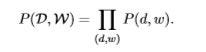
The main goal is to find a probabilistic model with latent or hidden topics that can generate the data which we observe in our document-term matrix. In mathematical terms, we want a model P(D, W) such that for any document d and word w in the corpus, P(d,w) corresponds to that entry in the document-term matrix.
So, pLSA is an advancement to LSA. It is a statistical technique for the analysis of two-mode and co-occurrence data.
Latent Variable Model for pLSA
Here we describe the two parametrizations for pLSA:
Parametrization -1
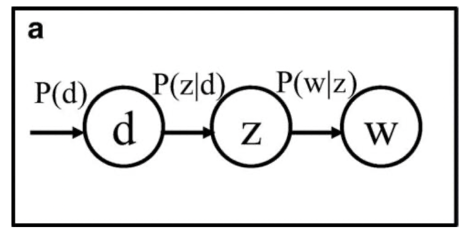
In this parametrization, we sample a document first then based on the document we sample a topic, and based on the topic we sample a word, which means d and w are conditionally independent given a hidden topic ‘z’.
The pictorial representation of this parametrization is as follows:
As discussed earlier, the topics are hidden variables. The only things we see are the words and the set of documents. So, In this framework, we have to find the relation between the hidden variables and the observed variables.
As we discussed the assumptions of the topic model, pLSA adds a probabilistic spin to these assumptions in the following way:
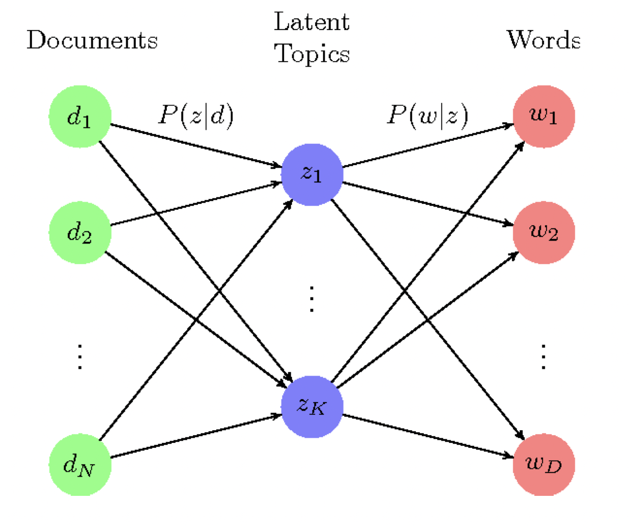
- Given a document d, a topic z is present in that selected document with probability P(z|d)
- Given a topic z, word w is drawn from the topic z with probability P(w|z)
Here we associate z with (d,w) and described a generative process where we select a document, then a topic, and finally a word from that topic. Formally,
1. We select a document from the corpus with a probability P(d)
2. For every word in the selected document dn, and word wi
- Select a topic zi from a conditional distribution with a probability P(z|dn).
- Select a word with a probability P(w|zi)
Before diving into the mathematical equations, let’s discuss the two main assumptions this model makes.
Assumption-1(Bag of Words)
As we discussed while learning the text vectorization techniques that the word ordering in the vocabulary doesn’t matter. In simple words, the joint variable (d,w) is sampled independently.
Assumption-2(Conditional Independence)
It is one of the key assumptions that we make while formulating the theory is that the words and the documents are conditionally independent. Focus on the word conditionally. This implies
P(w,d|z) = P(w|z)*P(d|z)
The model under the above-stated discussion can be specified in the following manner:
![]()
Now,
![]()
![]()
By using the assumption of conditional independence, we have:
![]()
Now with the help of Bayes Rule, we get:
![]()
Now, as we know that we have to determine the P(D) directly from our corpus. Therefore, we reduce the above expression to the following expression with the help of basic rules of conditional probability. Therefore, the joint probability of seeing a given document and word together is:
What does the expression on the right side of the above equation represent?
The right-hand side of the above equation tells us that how likely it is to observe some document and then based upon the distribution of topics in that document, how likely it is to find a certain word within that document. This is the exact interpretation of that component in the equation.
Other pictorial representation which definitely gives a good clarity about this parametrization:
What are the Parameters of this model?
The two main parameters in the model are as follows:
P(w|z): There is (M-1)*K of them. How? for every z we have M words.
The question is why we subtract 1 from the total number of words since the sum of these M probabilities should be 1, so we lose one degree of freedom, that’s why we have written (M-1) instead of M.
P(z|d): There are (K-1)*N parameters to determine.
Both these parameters are modeled as multinomial distributions and can be trained using the expectation-maximization algorithm.
Short Recap of Expectation-Maximization Algorithm
EM is a method of finding the likeliest parameter estimates for a model which depends on unobserved, latent variables (in our case, the latent variables are topics).
EM algorithm has the following two steps:
- Step-1: This step is known as the expectation (E) step, where posterior probabilities are computed for the latent variables,
- Step-2: This step is known as the maximization (M) step, where parameters are updated according to the likelihood function.
If you want to learn more about EM Algorithm, then refer to the following link:
Read the Article for EM Algorithm
Homework Problem
Here in the above section, we not discussed the objective function for the above parametrization for the EM algorithm. As your homework, you have to find out what is the objective function and log-likelihood function for the above model?
Note: You can take references from the paper, which I have given in the last section of the article.
Parametrization -2
In this parametrization, we are starting with the topic with P(z), and then independently generating the document with P(d|z) and the word with P(w|z).
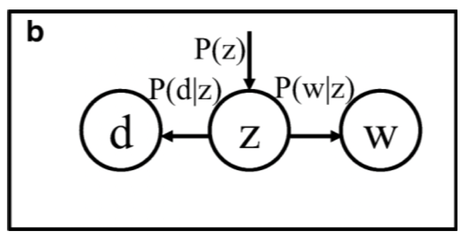
You can see the differences between this parametrization from the following diagram:
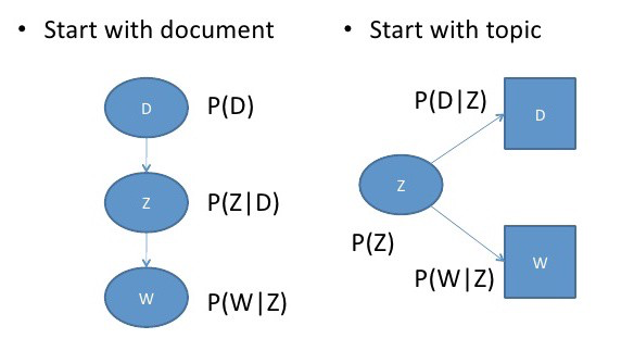
Image Source: Google Images
Interestingly, in this parametrization, P(D, W) can be equivalently parameterized using a different set of 3 parameters:
We can also look at the equivalency of the model as a generative process. This parametrization is more interesting than the first one since we can see a direct parallel between our pLSA model and our LSA model:
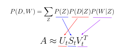
Image Source: Google Images
Now, a question comes to mind:
What do the different probabilities in this parametrization represent?
P(Z): The probability of our topic corresponds to the diagonal matrix of our singular topic probabilities,
P(D|Z): The probability of our document given the topic corresponds to our document-topic matrix U, and
P(W|Z): The probability of our word given the topic corresponds to our term-topic matrix V.
So what does that tell us?
Although it looks quite different and tackles the problem in a very different manner, and pLSA just adds a probabilistic treatment of topics and words on the top of LSA. Therefore, it is a far more flexible model but still faces the following issues.
- Since we have no parameters to model the probability P(D), so we don’t know how to assign probabilities to new documents.
- The number of parameters involved in the pLSA grows linearly with the number of documents we have, so it is prone to overfitting.
In general, when people are looking for a topic model beyond the baseline performance LSA gives, they try LDA, which is the most common type of topic model, and LDA is the extension of pLSA to overcome these issues.
Test Your Previous Knowledge
1. Which of the following are the instances of stemming according to Porter Stemmer?
- programer -> program
- programing -> program
- programmers -> program
- programmably -> program
2. According to Porter Stemmer, “python” cannot be the base form for which of the following word?
- pythoned
- pythoning
- pythonly
- pythoner
3. While preprocessing the text for POS tagging which of the following techniques will affect the POS tags?
- Case Folding
- Lemmatization
- Both
- None of the above
4. Stemming refers to the removal of suffices by a simple rule-based approach. Which of the following options demonstrates the stemming of words?
- was, am, is, are -> be
- helped, helps -> help
- troubled, troubling, trouble -> trouble
- friend, friendship, friends, friendships -> friend
Matrix Factorization model for pLSA
The matrix Factorization Model is an alternative way to represent pLSA.
Consider a document-word matrix of shape N × M, where N represents the number of documents and M represents the dictionary size. The elements of the matrix represent the counts of the occurrences of a word in a document. The element ((j, i) ) in a matrix becomes one if a word wi occurs once in the document dj.
The matrix formed above is a sparse matrix since most of the elements are 0.
For Example, Let’s have a document of 10 words and a dictionary having 1000 words. Then, 990 elements of the row will have the value 0. Such a matrix is called a Sparse Matrix.
Matrix Factorization breaks this matrix (let’s call it A) into lower dimension matrices with the help of Singular Value Decomposition.
![]()
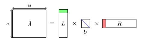
Image Source: Google Images
The shapes of the matrices L, U, and R are N × K, K × K, and K × M respectively.
Matrix U is a diagonal matrix with diagonal values equals to the square root of the eigenvalues of AAT. For any given k, you select the first k rows of L, the first k elements of U and the first k columns of R. And k represents the number of topics we want.
Remember this model is not very different from the Latent Variable Model.
How to interpret the above three matrices related to probabilities?
L matrix – This matrix contains the document probabilities P(d|z)
U matrix – This is a diagonal matrix that contains the prior probabilities of the topics P(z)
R matrix – This matrix corresponds to the word probability P(w|z)
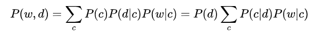
So if you do the multiplication of all the above described three matrices, then you actually do what the below equation says —
![]()
Note that the elements of all these three matrices cannot be negative as they represent probabilities. Hence, to decompose the A matrix, we can take the help of the Non-Negative Matrix Factorization, which we completed in the previous part of this Blog Series.
Advantages of pLSA
1. It models word-document co-occurrences as a mixture of conditionally independent multinomial distributions.
2. It is considered as a mixture model instead of a clustering model.
3. The results of pLSA have a clear probabilistic interpretation.
4. It also allows for model combination.
Disadvantages of pLSA
1. Potentially higher computational complexity.
2. EM algorithm gives local maximum instead of Global Maximum.
3. It is prone to overfitting.
4. It is not a well-defined generative model for new documents.
If you want to learn more about the pLSA, then read the following paper:
Read the Paper
This ends our Part-17 of the Blog Series on Natural Language Processing!
Other Blog Posts by Me
You can also check my previous blog posts.
Previous Data Science Blog posts.
Here is my Linkedin profile in case you want to connect with me. I’ll be happy to be connected with you.
For any queries, you can mail me on Gmail.
End Notes
Thanks for reading!
I hope that you have enjoyed the article. If you like it, share it with your friends also. Something not mentioned or want to share your thoughts? Feel free to comment below And I’ll get back to you. 😉
I am a B.Tech. student (Computer Science major) currently in the pre-final year of my undergrad. My interest lies in the field of Data Science and Machine Learning. I have been pursuing this interest and am eager to work more in these directions. I feel proud to share that I am one of the best students in my class who has a desire to learn many new things in my field.


