This article was published as a part of the Data Science Blogathon
This article contains Knowledge Distillation Theory and Code Walk-Through for its implementation on a business problem to classify x-ray images for pneumonia detection.

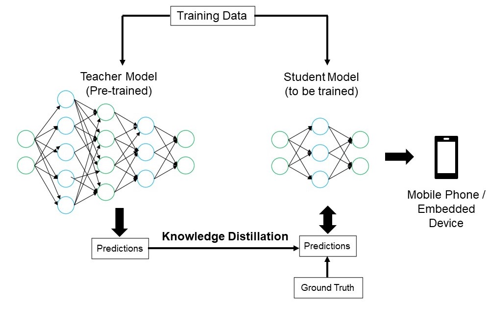
What is Knowledge Distillation?
Knowledge Distillation aims to transfer knowledge from a large deep learning model to a small deep learning model. Here size is in the context of the number of parameters present in the model which directly relates to the latency of the model.
Knowledge distillation is therefore a method to compress the model while maintaining accuracy. Here the bigger network which gives the knowledge is called a Teacher Network and the smaller network which is receiving the knowledge is called a Student Network.
Why make the Model Lighter?
Neural networks have been tremendously successful in diverse applications. Generally, the size of the Neural networks is huge (millions/billons parameters), which requires systems with high memory and computation power in order to train/deploy them.
In many applications, the model needs to be deployed on systems that have low computational power such as mobile devices, edge devices. For example, in the medical field, limited computation power systems (example: POCUS – Point of Care Ultrasound) are used in remote areas where it is required to run the models in real-time. From both time(latency) and memory (computation power) it is desirable to have ultra-lite and accurate deep learning models.
But ultra-lite (a few thousand parameters) models may not give us good accuracy. This is where we utilize Knowledge Distillation, taking help from the teacher network. It basically makes the model lite while maintaining accuracy.
Knowledge Distillation Steps
Below are the steps for Knowledge distillation:
1) Define Teacher Network and Student Network: The teacher (millions/billion parameters) and student (a few thousand parameters) networks are defined.
2) Train the teacher network fully: The teacher network is first trained separately till full convergence. Here the loss function can be any loss function based on the problem statement.
3) Train the student network intelligently in coordination with the teacher network: The student network is trained in coordination with the fully trained teacher network. Here forward propagation is done on both teacher and student networks and backpropagation is done on the student network. There are two loss functions defined. One is student loss and distillation loss function. These loss functions are explained in the next paragraph of this article.
Knowledge Distillation Mathematical Equations:
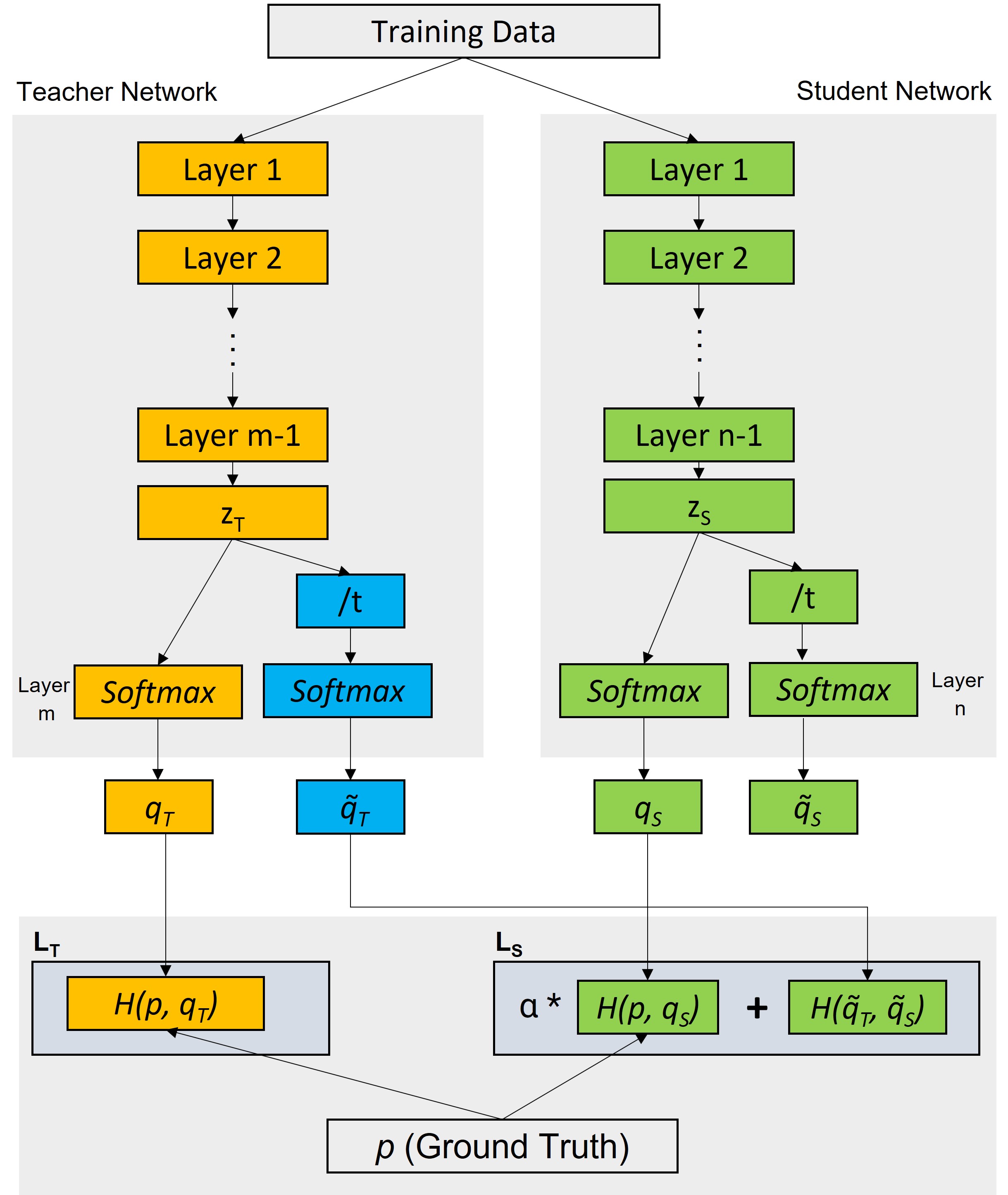
Loss Functions for teacher and student networks are defined as below:
Teacher Loss LT: (between actual lables and predictions by teacher network)
LT = H(p,qT)
Total Student Loss LTS :LTS = α * Student Loss + Distallation Loss
LTS = α* H(p,qs) + H(q̃T, q̃S)
Where,
Distillation Loss = H(q̃T, q̃S)Student Loss = H(p,qS)
Here:
H : Loss function (Categorical Cross Entropy or KL Divergence)zT and zS : pre-softmax logitsq̃T : softmax(zT/t)q̃S: softmax(zS/t)alpha (α) and temperature (t) are hyperparameters.Temperature t is used to reduce the magnitude difference among the class likelihood values.
These mathematical equations are taken from reference [3].
End to End Case Study
Here we will look at a case study where we will implement the knowledge distillation concept in an image classification problem for pneumonia detection.
About Data:
Dataset is taken from https://data.mendeley.com/datasets/rscbjbr9sj/2.
The dataset contains chest x-ray images. Each image can belong to one of three classes:
1) Normal
2) PNEUMONIA_BACTERIA or BACTERIA
3) PNEUMONIA_VIRUS or VIRUS
Let’s get started!!
Importing Required Libraries:
import numpy as np
import matplotlib.pyplot as plt
import os
import pandas as pd
import glob
import shutil
import tensorflow as tf
from tensorflow.keras.models import Model
from tensorflow.keras.layers import Conv2D, Dropout, MaxPool2D, BatchNormalization, Input, Conv2DTranspose, Concatenate
from tensorflow.keras.losses import SparseCategoricalCrossentropy, CategoricalCrossentropy
from tensorflow.keras.optimizers import Adam
from tensorflow.keras.callbacks import EarlyStopping, ModelCheckpoint
import matplotlib.pyplot as plt
from tensorflow.keras.preprocessing.image import ImageDataGenerator
import cv2
from sklearn.model_selection import train_test_split
import random
import h5py
from IPython.display import display
from PIL import Image as im
import datetime
import random
from tensorflow.keras import layers
Downloading the data
The data set is huge. I have randomly selected 1000 images for each class and kept 800 images in train data, 100 images in the validation data, and 100 images in test data for each of the classes. I had zipped this and uploaded this selected data into my google drive.
| S. No. | Class | Train | Test | Validation |
| 1. | Normal | 800 | 800 | 800 |
| 2. | BACTERIA | 100 | 100 | 100 |
| 3. | VIRUS | 100 | 100 | 100 |
Downloading the data from google drive to google colab:
#downloading the data and unzipping it
from google.colab import drive
drive.mount('/content/drive')
!unzip "/content/drive/MyDrive/data_xray.zip" -d "/content/"
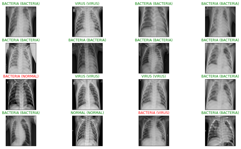
Visualizing the images
We will now look at some images from each of the classes.
for i, folder in enumerate(os.listdir(train_path)):
    for j, img in enumerate(os.listdir(train_path+"/"+folder)):
        filename = train_path+"/"+folder + "/" + img
        img= im.open(filename)
        ax = plt.subplot(3,4,4*i+j+1)
        ax.set_xlabel(folder+ ' '+ str(img.size[0]) +'x'+ str(img.size[1]))
        plt.imshow(img, 'gray')
        ax.set_xlabel(folder+ ' '+ str(img.size[0]) +'x'+ str(img.size[1]))
        ax.axes.xaxis.set_ticklabels([])
        ax.axes.yaxis.set_ticklabels([])
        #plt.axis('off')
        img.close()
        if j>2:
            break
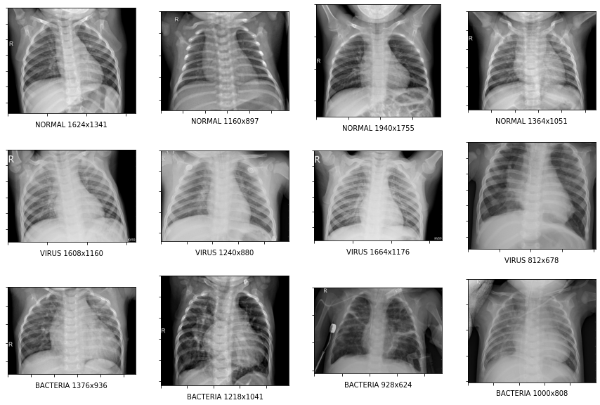
So above sample images suggest that each x-ray image can be of a different size.
Creating Data Generators
We will use Keras ImageDataGenerator for image augmentation. Image augmentation is a tool to get multiple transformed copies of an image. These transformations can be cropping, rotating, flipping. This helps in generalizing the model. This will also ensure that we get the same size (224×224) for each image. Below are the codes for train and validation data generators.
def trainGenerator(batch_size, train_path):
    datagen = ImageDataGenerator(rescale=1. / 255, rotation_range=5, shear_range=0.02, zoom_range=0.1,
                                       brightness_range=[0.7,1.3],  horizontal_flip=True,
                                         vertical_flip=True, fill_mode='nearest')
    train_gen = datagen.flow_from_directory(train_path, batch_size=batch_size,target_size=(224, 224), shuffle=True, seed=1, class_mode="categorical" )
    for image, label in train_gen:
        yield (image, label)
def validGenerator(batch_size, valid_path):
datagen = ImageDataGenerator(rescale=1. / 255, )
valid_gen = datagen.flow_from_directory(valid_path, batch_size=batch_size, target_size=(224, 224),shuffle=True, seed=1 )
for image, label in valid_gen:
yield (image, label)
Model 1: Teacher Network
Here we will use the VGG16 model and train it using transfer learning (based on the ImageNet dataset).
We will first define the VGG16 model.
from tensorflow.keras.applications.vgg16 import VGG16
base_model = VGG16(input_shape = (224, 224, 3), # Shape of our images
include_top = False, # Leave out the last fully connected layer
weights = ‘imagenet’)
Out of the total layers, We will make the first 8 layers untrainable:
len(base_model.layers)
for layer in base_model.layers[:8]:
layer.trainable = False
We will now add a dense layer with 512 “relu” activations units and a final softmax layer with 3 activation units since we have 3 classes. Also, we will use adam optimizer and categorical cross-entropy as loss functions.
x = layers.Flatten()(base_model.output)
# Add a fully connected layer with 512 hidden units and ReLU activation
x = layers.Dense(512, activation='relu')(x)
#x = layers.BatchNormalization()(x)
# Add a dropout rate of 0.5
x = layers.Dropout(0.5)(x)
x = layers.Dense(3)(x)   #linear activation to get pre-soft logits
model = tf.keras.models.Model(base_model.input, x)
opti = Adam(learning_rate=1e-4, beta_1=0.9, beta_2=0.999, epsilon=1e-08, decay=0.001)
model.compile(optimizer = opti, loss = tf.keras.losses.CategoricalCrossentropy(from_logits=True), metrics='acc')
model.summary()
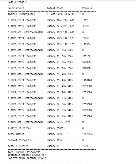
As we can see, there are 27M parameters in the teacher network.
One important point to note here is that the last layer of the model does not have any activation function (i.e. it has default linear activation). Generally, there would be a softmax activation function in the last layer as this is a multi-class classification problem but here we are using the default linear activation function to get pre-softmax logits. Because these pre-softmax logits will be used along with the student network’s pre-softmax logits in the distillation loss function.
Hence, we are using from_logits = True in the CategoricalCrossEntropy loss function. This means that the loss function will calculate the loss directly from the logits. If we had used softmax activation, then it would have been from_logits = False.
We will now define a callback for the early stopping of the model and run the model.
Running the model:
earlystop = EarlyStopping(monitor='val_acc', patience=5, verbose=1)
filepath="model_save/weights-{epoch:02d}-{val_accuracy:.4f}.hdf5"
checkpoint = ModelCheckpoint(filepath=filepath, monitor='val_acc', verbose=1, save_best_only=True, mode='max')
callbacks = [earlystop ]
vgg_hist = model.fit(train_generator, validation_data = validation_generator, validation_steps=10,
                    steps_per_epoch = 90, epochs = 50, callbacks=callbacks)
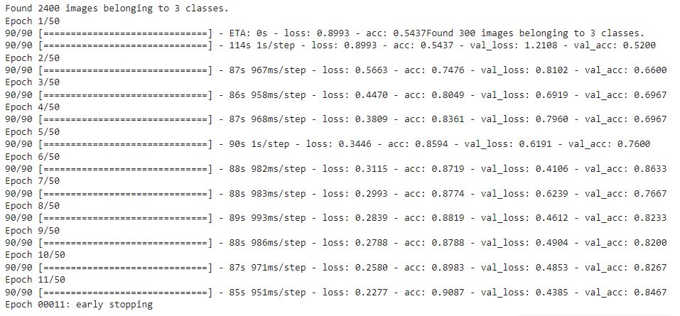
Checking the accuracy and loss for each epoch:
import matplotlib.pyplot as plt
plt.figure(1)
# summarize history for accuracy
plt.subplot(211)
plt.plot(vgg_hist.history['acc'])
plt.plot(vgg_hist.history['val_acc'])
plt.title('teacher model accuracy')
plt.ylabel('accuracy')
plt.xlabel('epoch')
plt.legend(['train', 'valid'], loc='lower right')
 # summarize history for loss
plt.subplot(212)
plt.plot(vgg_hist.history['loss'])
plt.plot(vgg_hist.history['val_loss'])
plt.title('teacher model loss')
plt.ylabel('loss')
plt.xlabel('epoch')
plt.legend(['train', 'valid'], loc='upper right')
plt.show()
Now we will evaluate the model on the test data:
# First, we are going to load the file names and their respective target labels into a numpy array!
from sklearn.datasets import load_files
import numpy as np
test_dir = '/content/test'
def load_dataset(path):
    data = load_files(path)
    files = np.array(data['filenames'])
    targets = np.array(data['target'])
    target_labels = np.array(data['target_names'])
    return files,targets,target_labels
x_test, y_test,target_labels = load_dataset(test_dir)
from keras.utils import np_utils
y_test = np_utils.to_categorical(y_test,no_of_classes)
# We just have the file names in the x set. Let's load the images and convert them into array.
from keras.preprocessing.image import array_to_img, img_to_array, load_img
def convert_image_to_array(files):
    images_as_array=[]
    for file in files:
        # Convert to Numpy Array
        images_as_array.append(tf.image.resize(img_to_array(load_img(file)), (224, 224)))
    return images_as_array
x_test = np.array(convert_image_to_array(x_test))
print('Test set shape : ',x_test.shape)
x_test = x_test.astype('float32')/255
# Let's visualize test prediction.
y_pred_logits = model.predict(x_test)
y_pred = tf.nn.softmax(y_pred_logits)
# plot a raandom sample of test images, their predicted labels, and ground truth
fig = plt.figure(figsize=(16, 9))
for i, idx in enumerate(np.random.choice(x_test.shape[0], size=16, replace=False)):
    ax = fig.add_subplot(4, 4, i + 1, xticks=[], yticks=[])
    ax.imshow(np.squeeze(x_test[idx]))
    pred_idx = np.argmax(y_pred[idx])
    true_idx = np.argmax(y_test[idx])
    ax.set_title("{} ({})".format(target_labels[pred_idx], target_labels[true_idx]),
                 color=("green" if pred_idx == true_idx else "red"))
Calculating the accuracy of the test dataset:
print(model.metrics_names)
loss, acc = model.evaluate(x_test, y_test, verbose = 1)
print('test loss = ', loss)
print('test accuracy = ',acc)
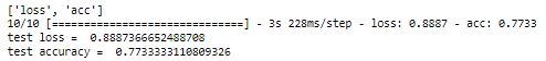
We have achieved 77% accuracy in the test dataset with Teacher Network. Now we will define the student network.
Model 2 –Student Model with Knowledge Distillation
This is the creative part here. We can define any student network and experiment with it. The idea here is to define a network that is similar to the teacher network but with a very less number of parameters. Input and Output layers would remain the same as the teacher network.
The student network defined here has a series of 2D convolutions and max-pooling layers just like our teacher network VGG16. The only difference is that number of Convolutions filters in the student network is very less in each layer as compared to the teacher network. This would make us achieve our goal to have a very less number of weights (parameters) to be learned in the student network during training.
Defining the student network:
# import necessary layers
from tensorflow.keras.layers import Input, Conv2D
from tensorflow.keras.layers import MaxPool2D, Flatten, Dense, Dropout
from tensorflow.keras import Model
# input
input = Input(shape =(224,224,3))
# 1st Conv Block
x = Conv2D (filters =8, kernel_size =3, padding ='valid', activation='relu')(input)
x = Conv2D (filters =8, kernel_size =3, padding ='valid', activation='relu')(x)
x = MaxPool2D(pool_size =2, strides =2, padding ='valid')(x)
# 2nd Conv Block
x = Conv2D (filters =16, kernel_size =3, padding ='valid', activation='relu')(x)
x = Conv2D (filters =16, kernel_size =3, padding ='valid', activation='relu')(x)
x = MaxPool2D(pool_size =2, strides =2, padding ='valid')(x)
# 3rd Conv block
x = Conv2D (filters =32, kernel_size =3, padding ='valid', activation='relu')(x)
x = Conv2D (filters =32, kernel_size =3, padding ='valid', activation='relu')(x)
#x = Conv2D (filters =32, kernel_size =3, padding ='valid', activation='relu')(x)
x = MaxPool2D(pool_size =2, strides =2, padding ='valid')(x)
# 4th Conv block
x = Conv2D (filters =64, kernel_size =3, padding ='valid', activation='relu')(x)
x = Conv2D (filters =64, kernel_size =3, padding ='valid', activation='relu')(x)
#x = Conv2D (filters =64, kernel_size =3, padding ='valid', activation='relu')(x)
x = MaxPool2D(pool_size =2, strides =2, padding ='valid')(x)
# 5th Conv block
x = Conv2D (filters =64, kernel_size =3, padding ='valid', activation='relu')(x)
x = Conv2D (filters =64, kernel_size =3, padding ='valid', activation='relu')(x)
#x = Conv2D (filters =64, kernel_size =3, padding ='valid', activation='relu')(x)
x = MaxPool2D(pool_size =2, strides =2, padding ='valid')(x)
# Fully connected layers
x = Flatten()(x)
#x = Dense(units = 1028, activation ='relu')(x)
x = Dense(units = 256, activation ='relu')(x)
x = Dropout(0.5)(x)
output = Dense(units = 3)(x)   #last layer with linear activation
# creating the model
s_model_1 = Model (inputs=input, outputs =output)
s_model_1.summary()
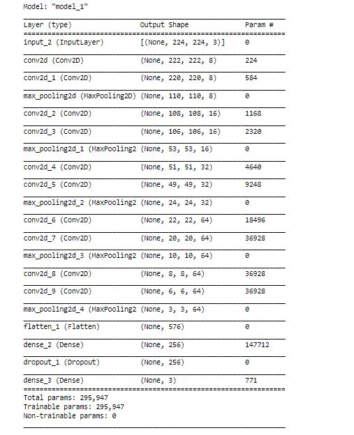
Note that the number of parameters here is only 296k as compared to what we got in the teacher network (27M).
Now we will define the distiller. Distiller is a custom class that we will define in Keras in order to establish coordination/communication with the teacher network.
This Distiller Class takes student-teacher networks, hyperparameters (alpha and temperature as mentioned in the first part of this article), and the train data (x,y) as input. The Distiller Class does forward propagation of teacher and student networks and calculates both the losses: Student Loss and Distillation Loss. Then the backpropagation of the student network is done and weights are updated.
Defining the Distiller:
class Distiller(keras.Model):
    def __init__(self, student, teacher):
        super(Distiller, self).__init__()
        self.teacher = teacher
        self.student = student
    def compile(
        self,
        optimizer,
        metrics,
        student_loss_fn,
        distillation_loss_fn,
        alpha=0.5,
        temperature=2,
    ):
        """ Configure the distiller.
        Args:
            optimizer: Keras optimizer for the student weights
            metrics: Keras metrics for evaluation
            student_loss_fn: Loss function of difference between student
                predictions and ground-truth
            distillation_loss_fn: Loss function of difference between soft
                student predictions and soft teacher predictions
            alpha: weight to student_loss_fn and 1-alpha to distillation_loss_fn
            temperature: Temperature for softening probability distributions.
                Larger temperature gives softer distributions.
        """
        super(Distiller, self).compile(optimizer=optimizer, metrics=metrics)
        self.student_loss_fn = student_loss_fn
        self.distillation_loss_fn = distillation_loss_fn
        self.alpha = alpha
        self.temperature = temperature
    def train_step(self, data):
        # Unpack data
        x, y = data
        # Forward pass of teacher
        teacher_predictions = self.teacher(x, training=False)
        #model = ...  # create the original model
        teacher_predictions = self.teacher(x, training=False)
        with tf.GradientTape() as tape:
            # Forward pass of student
            # Forward pass of student
            student_predictions = self.student(x, training=True)
            # Compute losses
            student_loss = self.student_loss_fn(y, student_predictions)
            distillation_loss = self.distillation_loss_fn(
                tf.nn.softmax(teacher_predictions / self.temperature, axis=1),
                tf.nn.softmax(student_predictions / self.temperature, axis=1),
            )
            loss = self.alpha * student_loss +  distillation_loss
        # Compute gradients
        trainable_vars = self.student.trainable_variables
        gradients = tape.gradient(loss, trainable_vars)
        # Update weights
        self.optimizer.apply_gradients(zip(gradients, trainable_vars))
        # Update the metrics configured in `compile()`.
        self.compiled_metrics.update_state(y, student_predictions)
        # Return a dict of performance
        results = {m.name: m.result() for m in self.metrics}
        results.update(
            {"student_loss": student_loss, "distillation_loss": distillation_loss}
        )
        return results
    def test_step(self, data):
        # Unpack the data
        x, y = data
        # Compute predictions
        y_prediction = self.student(x, training=False)
        # Calculate the loss
        student_loss = self.student_loss_fn(y, y_prediction)
        # Update the metrics.
        self.compiled_metrics.update_state(y, y_prediction)
        # Return a dict of performance
        results = {m.name: m.result() for m in self.metrics}
        results.update({"student_loss": student_loss})
        return results
Now we will initialize and compile the distiller. Here for the student loss, we are using the Categorical cross-entropy function and for distillation loss, we are using the KLDivergence loss function.
KLDivergence loss function is used to calculate the distance between two probability distributions. By minimizing the KLDivergence we are trying to make student network predict similar to teacher network.
Compiling and Running the Student Network Distiller:
# Initialize and compile distiller
distiller = Distiller(student=s_model_1, teacher=model)
distiller.compile(
optimizer=Adam(learning_rate=1e-4, beta_1=0.9, beta_2=0.999, epsilon=1e-08, decay=0.001),
metrics=['acc'],
student_loss_fn=CategoricalCrossentropy(from_logits=True),
distillation_loss_fn=tf.keras.losses.KLDivergence(),
alpha=0.5,
temperature=2,
)
# Distill teacher to student
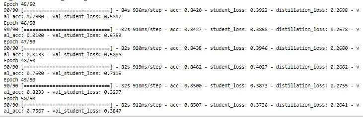
distiller_hist = distiller.fit(train_generator, validation_data = validation_generator, epochs=50, validation_steps=10,
steps_per_epoch = 90)
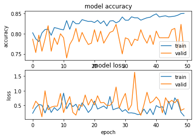
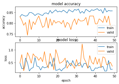
Checking the plot of accuracy and loss for each epoch:
import matplotlib.pyplot as plt
plt.figure(1)
# summarize history for accuracy
plt.subplot(211)
plt.plot(distiller_hist.history['acc'])
plt.plot(distiller_hist.history['val_acc'])
plt.title('model accuracy')
plt.ylabel('accuracy')
plt.xlabel('epoch')
plt.legend(['train', 'valid'], loc='lower right')
 # summarize history for loss
plt.subplot(212)
plt.plot(distiller_hist.history['student_loss'])
plt.plot(distiller_hist.history['val_student_loss'])
plt.title('model loss')
plt.ylabel('loss')
plt.xlabel('epoch')
plt.legend(['train', 'valid'], loc='upper right')
plt.show()
plt.tight_layout()
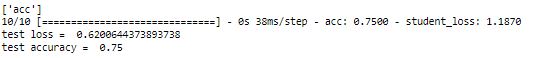
Checking accuracy on the test data:
print(distiller.metrics_names)
acc, loss = distiller.evaluate(x_test, y_test, verbose = 1)
print('test loss = ', loss)
print('test accuracy = ',acc)

We have got 74% accuracy on the test data. With the teacher network, we had got 77% accuracy. Now we will change the hyperparameter t, to see if we can improve the accuracy in the student network.
Compiling and Running the Distiller with t = 6:
# Initialize and compile distiller
distiller = Distiller(student=s_model_1, teacher=model)
distiller.compile(
optimizer=Adam(learning_rate=1e-4, beta_1=0.9, beta_2=0.999, epsilon=1e-08, decay=0.001),
metrics=['acc'],
student_loss_fn=CategoricalCrossentropy(from_logits=True),
#distillation_loss_fn=CategoricalCrossentropy(),
distillation_loss_fn=tf.keras.losses.KLDivergence(),
alpha=0.5,
temperature=6,
)
# Distill teacher to student
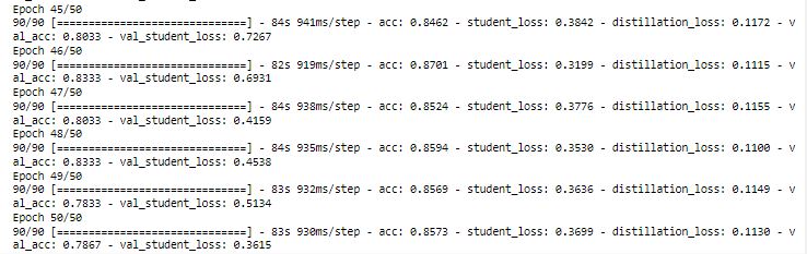
distiller_hist = distiller.fit(train_generator, validation_data = validation_generator, epochs=50, validation_steps=10,
steps_per_epoch = 90)
Plotting the loss and accuracy for each epoch:
import matplotlib.pyplot as plt
plt.figure(1)
# summarize history for accuracy
plt.subplot(211)
plt.plot(distiller_hist.history['acc'])
plt.plot(distiller_hist.history['val_acc'])
plt.title('model accuracy')
plt.ylabel('accuracy')
plt.xlabel('epoch')
plt.legend(['train', 'valid'], loc='lower right')
 # summarize history for loss
plt.subplot(212)
plt.plot(distiller_hist.history['student_loss'])
plt.plot(distiller_hist.history['val_student_loss'])
plt.title('model loss')
plt.ylabel('loss')
plt.xlabel('epoch')
plt.legend(['train', 'valid'], loc='upper right')
plt.show()
plt.tight_layout()
Checking the test accuracy:
print(distiller.metrics_names)
acc, loss = distiller.evaluate(x_test, y_test, verbose = 1)
print('test loss = ', loss)
print('test accuracy = ',acc)
With t = 6, we have got 75% accuracy which is better than what we got with t = 2.
This way, we can do more iterations by changing the values of hypermeters alpha (α) and temperature (t) in order to get better accuracy.
Model 3: Student Model without Knowledge Distillation
Now we will check the student model without Knowledge Distillation. Here there will be no coordination with the teacher network and there will be only one loss function i.e. Student Loss.
The student model remains the same as the previous model (Model 2). We will just run it without distillation.
Compiling and running the model:
opti = Adam(learning_rate=1e-4, beta_1=0.9, beta_2=0.999, epsilon=1e-08, decay=0.001)
s_model_2.compile(optimizer = opti, loss = tf.keras.losses.CategoricalCrossentropy(from_logits=True),metrics = ['acc'])
earlystop = EarlyStopping(monitor='val_acc', patience=5, verbose=1)
filepath="model_save/weights-{epoch:02d}-{val_accuracy:.4f}.hdf5"
checkpoint = ModelCheckpoint(filepath=filepath, monitor='val_acc', verbose=1, save_best_only=True, mode='max')
callbacks = [earlystop ]
s_model_2_hist = s_model_2.fit(train_generator, validation_data = validation_generator, validation_steps=10,
                    steps_per_epoch = 90, epochs = 50, callbacks=callbacks)
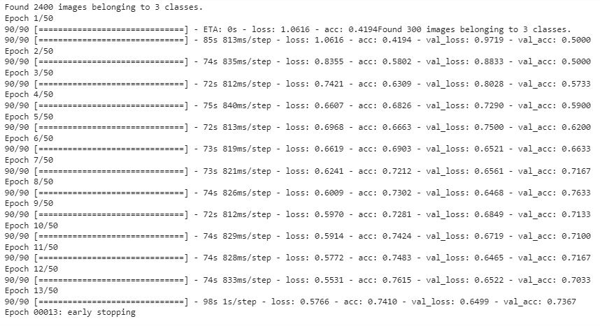
Our model stopped in 13 epochs as we had used early stop callback if there is no improvement in validation accuracy in 5 epochs.
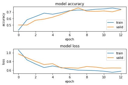
Plotting the loss and accuracy for each epoch:
import matplotlib.pyplot as plt
plt.figure(1)
# summarize history for accuracy
plt.subplot(211)
plt.plot(s_model_2_hist.history['acc'])
plt.plot(s_model_2_hist.history['val_acc'])
plt.title('model accuracy')
plt.ylabel('accuracy')
plt.xlabel('epoch')
plt.legend(['train', 'valid'], loc='lower right')
 # summarize history for loss
plt.subplot(212)
plt.plot(s_model_2_hist.history['loss'])
plt.plot(s_model_2_hist.history['val_loss'])
plt.title('model loss')
plt.ylabel('loss')
plt.xlabel('epoch')
plt.legend(['train', 'valid'], loc='upper right')
plt.tight_layout()
plt.show()
Checking the Test Accuracy:
print(s_model_2.metrics_names)
loss, acc = s_model_2.evaluate(x_test, y_test, verbose = 1)
print(‘test loss = ‘, loss)
print(‘test accuracy = ‘,acc)
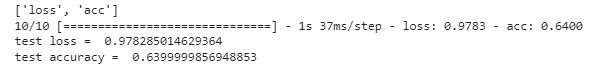
Here we are able to achieve 64% accuracy on the test data.
Result Summary:
Below is the comparison of all four models that are made in this case study:
| S. No. | Model | No. of Parameters | Hyperparameter | Test Accuracy | |
| 1 | Teacher Model | 27 M | – | 77% | |
| 2 | Student Model with Distillation | 296 k | α = 0.5, t = 2 | 74% | |
| 3 | Student Model with Distillation | 296 k | α = 0.5, t = 6 | 75% | |
| 4 |
|
296 k | – | 64% |
As seen from the above table, with Knowledge distillation, we have achieved 75% accuracy with a very lite neural network. We can play around with the hypermeters α and t to improve it further.
Conclusion
In this article, we saw that Knowledge Distillation can compress a Deep CNN while maintaining the accuracy so that it can be deployed on embedded systems that have less storage and computational power.
We used Knowledge Distillation on the Pneumonia detection problem from x-ray images. By distilling Knowledge from a Teacher Network having 27M parameters to a Student Network having only 0.296M parameters (almost 100 times lighter), we were able to achieve almost the same accuracy. With more hyperparameter iterations and ensembling of multiple students networks as mentioned in reference [3], the performance of the student model can be further improved.
References
1) Identifying Medical Diagnoses and Treatable Diseases by Image-Based Deep Learning 2018.
https://www.sciencedirect.com/science/article/pii/S0092867418301545
2) Dataset: Kermany, Daniel; Zhang, Kang; Goldbaum, Michael (2018), “Labeled Optical Coherence Tomography (OCT) and Chest X-Ray Images for Classification”, Mendeley Data, V2, doi: 10.17632/rscbjbr9sj.2
https://data.mendeley.com/datasets/rscbjbr9sj/2
3) Designing Lightweight Deep Learning Models for Echocardiography View Classification 2019.
https://www.researchgate.net/publication/331633115
4) https://keras.io/examples/vision/knowledge_distillation/
5) https://ramesharvind.github.io/posts/deep-learning/knowledge-distillation/
6) https://towardsdatascience.com/can-a-neural-network-train-other-networks-cf371be516c6
7) https://intellabs.github.io/distiller/knowledge_distillation.html
8) Jupyter Notebook Code file: https://github.com/vijendra-code/knowledge-distillation-pneumonia-detection
The media shown in this article is not owned by Analytics Vidhya and are used at the Author’s discretion.


Thanks for this tutorial. Please, I would like have a discussion with you on this topic and your kind help will be much appreciated. Thanks and I look forward to hearing from you. Kind regards, Charles
Hi I would like to know as to why the first 8 layers were no trained for the teacher model? also the github link to this code shows only the readme file, kindly let me know if there is another link to get the source code for this KD experiment? thanks!