10 Ways to Clean Data in an Excel Sheet

Every data analyst has had that sinking feeling when opening a new spreadsheet, seeing unformatted numbers, inconsistent entries, random blank cells, and duplicates everywhere! Cleaning up this data is essential to start working on it. Whether you’re putting together a quarterly report, consumer behaviour analysis, or trend forecasting, the quality of your interpretation depends on how well you’ve cleaned the data first. Cleaning data in Excel is not just a technical step; it’s the basic foundation that converts raw information into astute insights for businesses. In this article, I will explain to you what data cleaning is and guide you on how to remove duplicates and clean data in Excel.

What is Data Cleaning in Excel?

Cleaning data in Excel Sheets involves identifying and fixing errors, getting rid of inconsistencies, and removing duplicates and inaccuracies. Examining the raw data to identify and handle outliers – such as duplicate entries and missing values using Excel’s built-in functions and tools ensures more accurate and reliable results.

What are the Characteristics of Clean Data?

Clean data can be identified based on the following characteristics:

1. Accuracy: Data should reproduce the real value without giving room to errors.
2. Completeness: All necessary values are present, with very little missing.
3. Consistency: Similar data follows the same format throughout the dataset.
4. Uniformity: Units of measurement, abbreviations, and naming conventions should be standardized.
5. Uniqueness: There should be no unnecessary duplicate records in the dataset.
6. Validity: Data must fall within an acceptable range and meet the defined rules.
7. Timeliness: Data should be up to date and relevant to the time of analysis.

How to Clean Data in Excel Sheets?

In this section, we’ll explore some of the standard techniques used to clean data in Excel Sheets:

1. Remove Duplicates

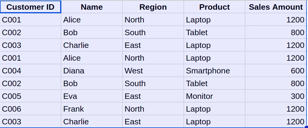
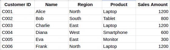
Duplicate records can seriously skew one’s analysis, giving false perceptions of volume or frequency. Suppose the same customer was counted twice in sales numbers; this would lead to a discrepancy in the entire dataset. Hence, it’s important to remove duplicates for accurate data analysis.

Steps to Remove Duplicates

1. Select the range of data (Including headers) to remove duplicates from.

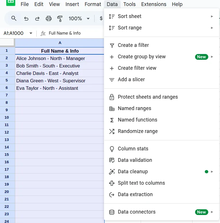
2. Go to the Data tab in the menu bar.

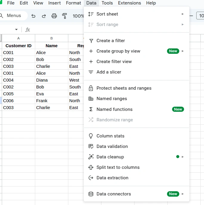
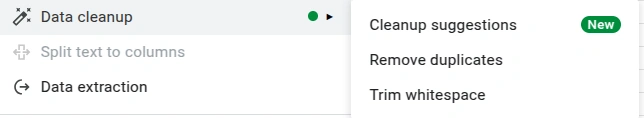
3. Click on Data cleanup and select Remove duplicates.

4. Here, you’ll get a pop-up to select the columns from which you wish to remove duplicate values. You can choose to select all or some specific columns only.

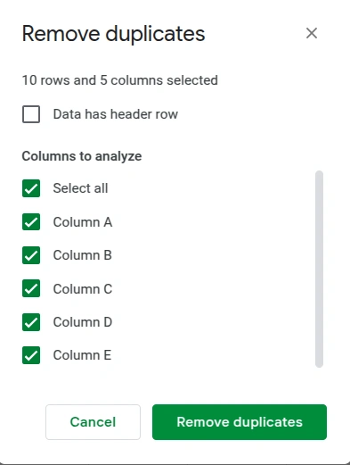
5. Click on Remove duplicates to get the duplicates removed.

Also Read: Microsoft Excel for Data Analysis

2. Standardize Formats

Inconsistent formatting is an obstacle to data analysis. Even elementary tasks, such as sorting, can fail when dates, numbers, or text use different formats or conventions, so it’s necessary to standardize the formats of the data.

Steps to Standardize Formats

1. Select the column or required range of data that you need to standardize, like in this example, we’ll be choosing the column containing dates.

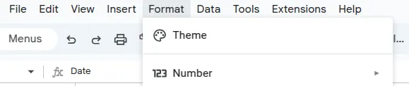
2. From the menu bar, go to Format and then choose Number.

3. Choose the format you want to follow from the list. Here we’ll select Date and it will convert the selected data to that format.

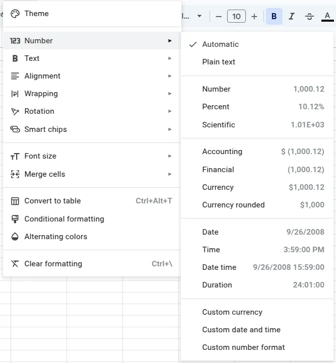
4. You have other formatting options that you can choose from as well.

3. Clean Text Data

Every text analysis starts with cleaning. Raw text data frequently contains inconsistencies like extra spaces, inappropriate cases, typos, or special symbols. This may interfere with grouping, filtering, or interpretation. Without sufficient cleaning, the most advanced methods or models will struggle to yield results of value.

Steps to Clean Text Data

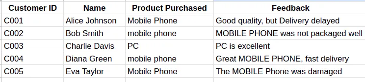
Let’s consider this dataset

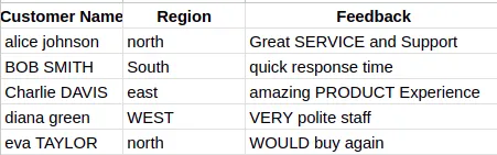
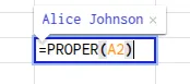
1. Capitalize the first letter of each word using the PROPER function. The formula of this function: =PROPER(cell)

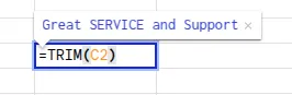
2. Remove the extra spaces present using the TRIM function. The formula is written as: =TRIM(cell)

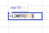
3. Convert text to either all uppercase or lowercase format using the “LOWER” & “UPPER” functions. The formula is written as: =LOWER(cell) or =UPPER(cell)

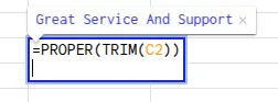
4. We can use the combination of two of these functions to clean the data more comprehensively. The formula for this is written as: =FIRST FUNCTION(SECOND FUNCTION(cell))

Also Read: Data Cleaning for Beginners – Why and How?

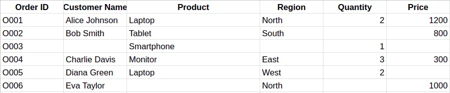
4. Fill Missing Values

There might be some cases where you’ll see missing values, and these values might create blind spots in your analysis. Filling your data with some random values is not the solution, but there are several ways to handle these gaps appropriately.

Steps to Fill Missing Values

Consider the following dataset

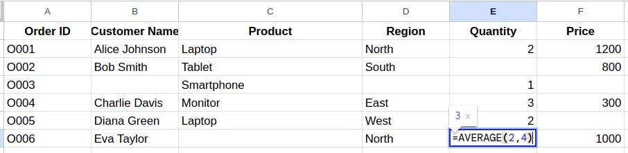
1. You can easily fill in missing numerical values using the AVERAGE formula. This will add the calculated average, which is a more realistic value within the existing range. The formula can be written as: =AVERGAGE(min,max)

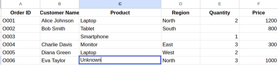
2. For categorical data, you can use logical assumptions like “Not Available” or “Unknown” wherever suitable.

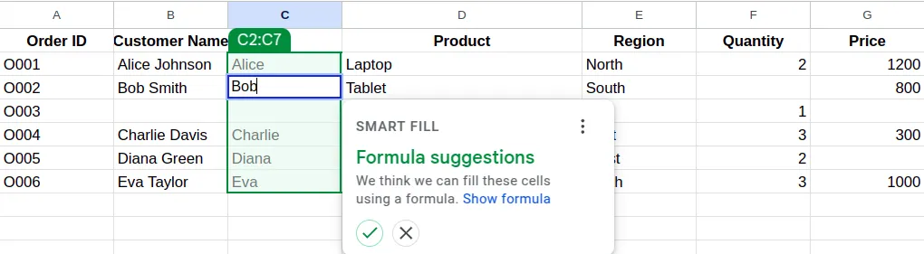
3. You can also use Smart Fill to detect patterns and then fill in missing values.

5. Validate the Data

Data validation is the process that controls and sets the rules for what can be entered into cells and what cannot. Using this to prevent errors is much easier than fixing those errors later.

Steps for Data Validation

1. Select the row or column with the data you need to validate.

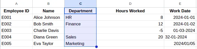
2. Go to the Data tab on the menu bar and select Data validation.

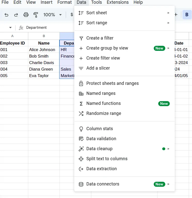
3. Choose the specific criteria of validation under the validation rule, such as whole numbers, dates, lists, etc.

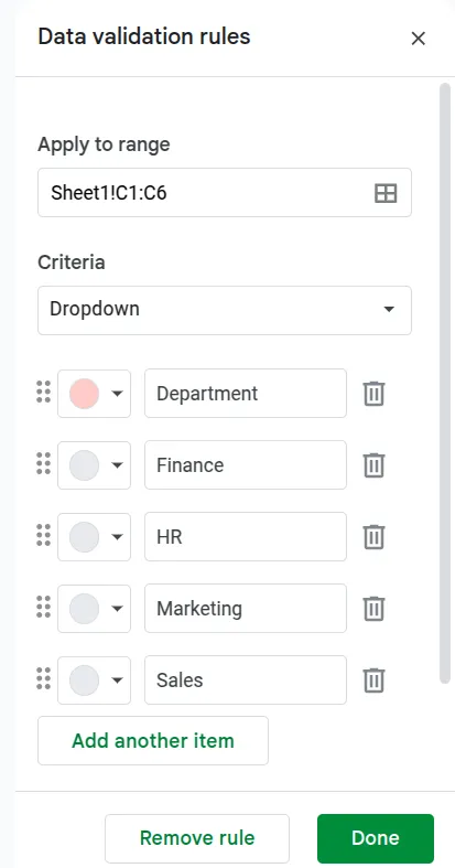
4. Then set the specific parameters or the various options that can be added in the cell, like date or time in a particular format, the name of departments, etc.

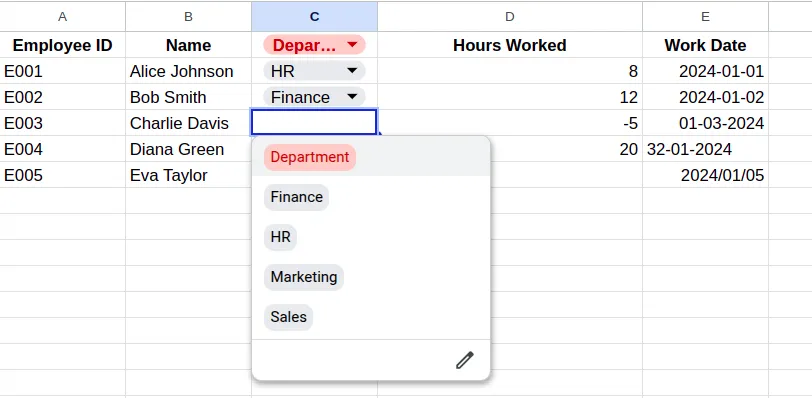
5. Once set, you will have your data validated.

Also Read: Advanced Microsoft Excel for Data Analysis

6. Apply Conditional Formatting

There will be some visual cues that might help us identify the potential issues in the data quickly by highlighting the values that meet specific criteria. For data cleaning purposes, they can basically highlight duplicate values, flag outliers, identify missing values, and mark the cells containing formulas with errors.

Steps for Conditional Formatting

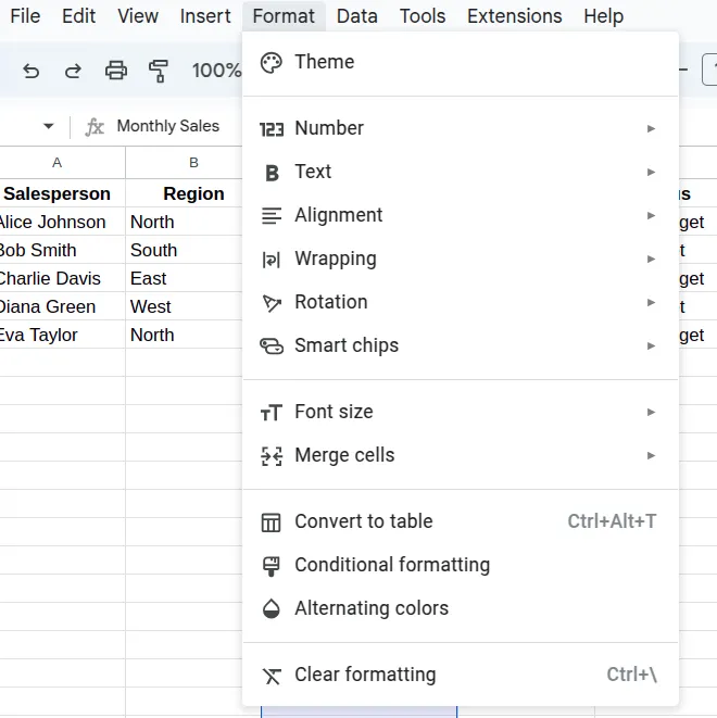
1. Select the range of the data you wish to clean.

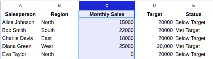
2. Go to the Format tab on the menu bar and choose the option Conditional formatting.

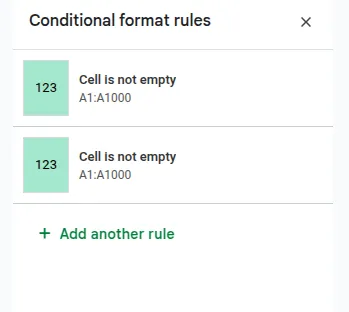
3. Choose the type of rule you want to apply (highlight cells rules, top/bottom rules, etc.)

4. Then define the formatting styles and the required conditions. For example, here I am applying ‘highlight cells in the specified column, which are greater than 2000, in red.’

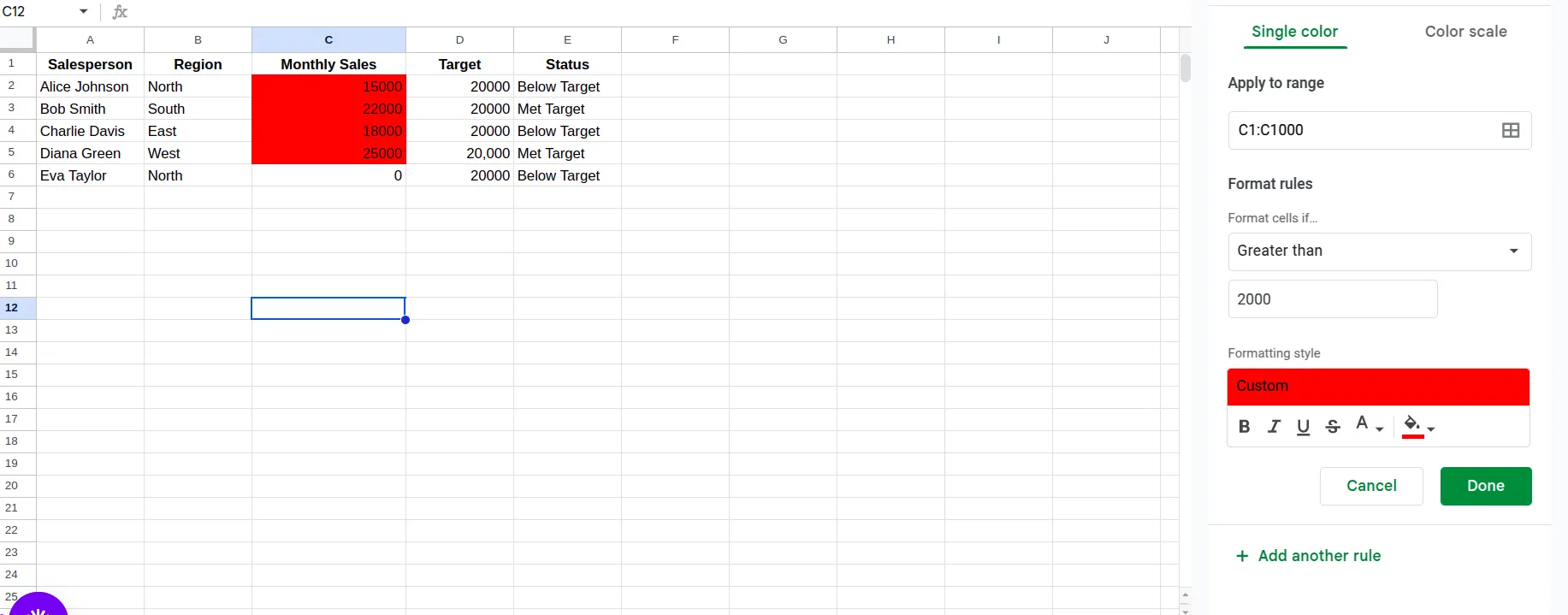
5. Once set, click on Done.

7. Power Query

There is an advanced data cleaning method called ‘Get & Transform’ which is available in newer versions of Microsoft Excel. It is used for more complex data cleaning purposes. It offers robust options for cleaning and reshaping the data before putting it into your spreadsheet.

If you’re using Excel 2016 or a later version, it comes with built-in Power Query functionality. Else, you can add it as an add-in in Excel 2010 and subsequent versions.

Steps to Use Power Query

1. Click on the Get Data button in the Power Query tab, and you’ll get a drop-down menu having numerous file types like csv file, webpages, etc.

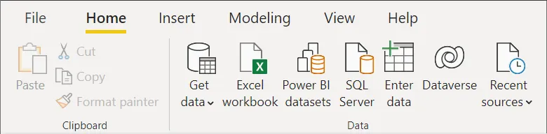
2. Choose your data source.

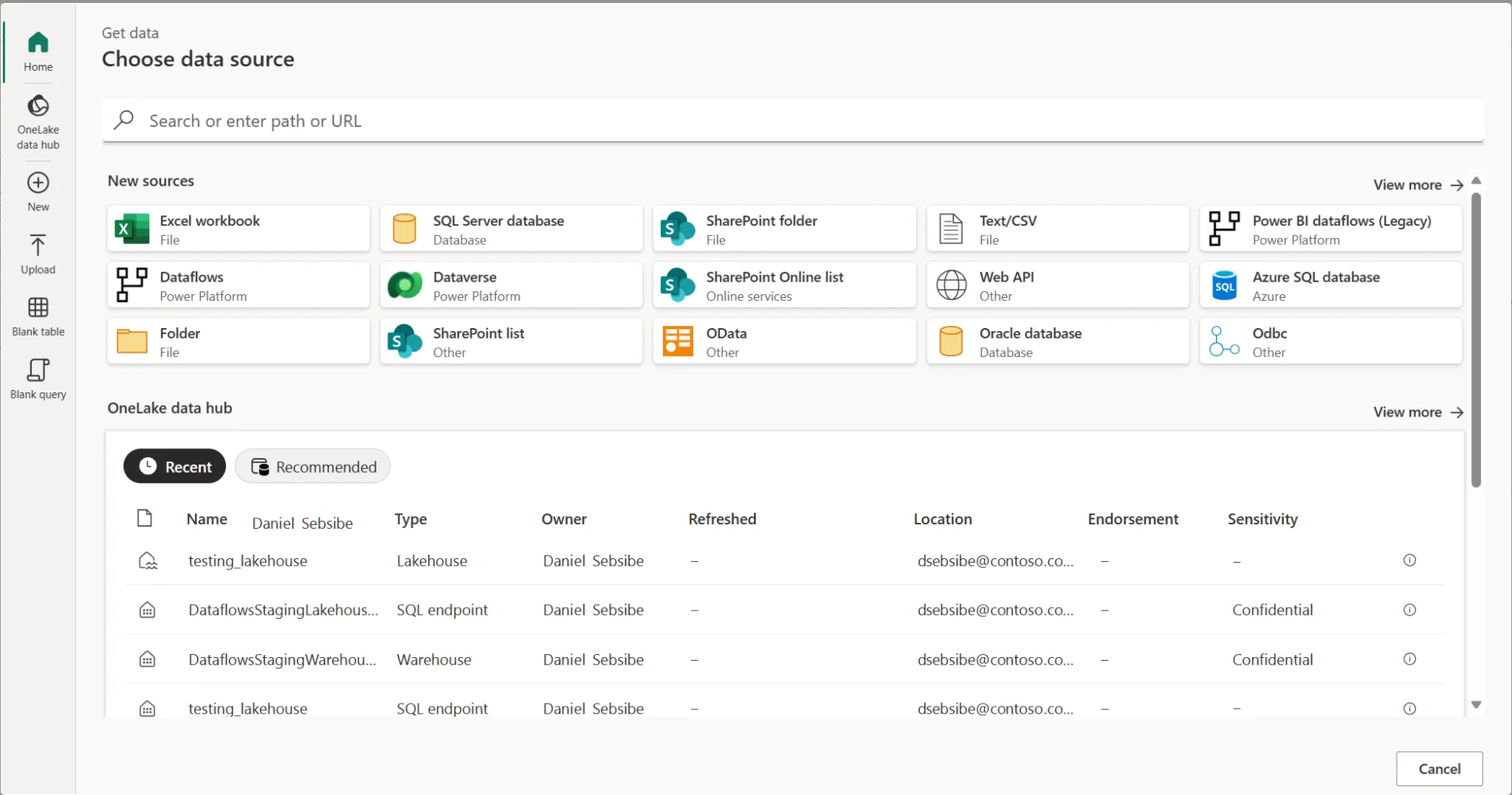
3. When a data source is chosen, Excel will prompt for a connection that requires certain information based on the type of source. For a source such as a file, you’ll be asked to provide the file path (browsing to the location). On the other hand, for a web source, you’ll need to enter a valid URL.
4. Once the source is specified for loading, the following option may arise. You may be requested to pick a sheet, table, or range and then enter your credentials to authorize.
5. Make sure to review the columns while selecting only those that you really require. Either load or transform your data for it to show up in the Power Query Editor, where further cleaning takes place.

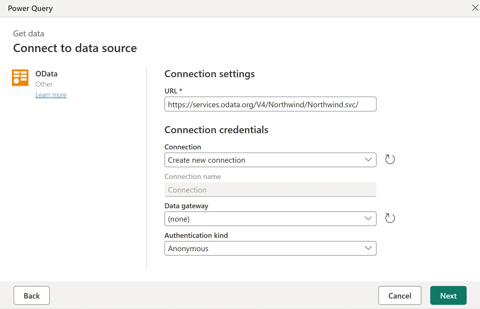
6. You can even filter your data according to your requirements using Power Query. For example, you can deal with missing data or remove columns by following these steps:

• Go to the Home tab in the Power Query editing window.
• Select the data you want to deal with.
• Choose the Remove columns option from the menu, and you’ll have your output.

8. Find and Replace Feature

Find and replace is an easier way to make consistent changes across large amounts of data without any disruption.

Steps to Use the Find and Replace Feature

1. Choose Edit from the menu bar and then click on Find and replace. Alternatively, you can easily use the shortcut Ctrl+H.

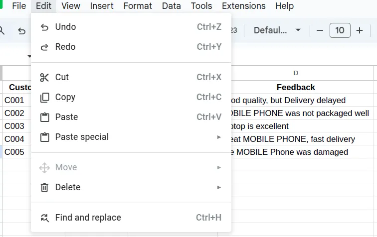
2. Enter the text that you want to find, and then enter the replacement text.

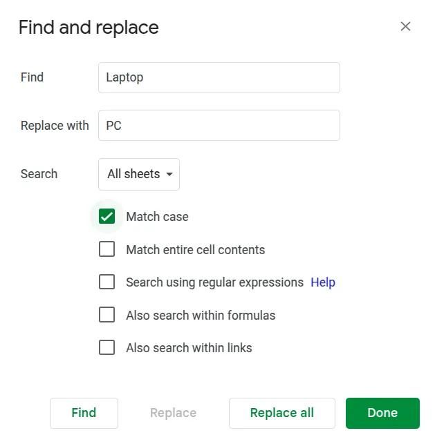
3. You may use options like Match case for precision, as shown in the above image.
4. Click on Replace to control the changes individually or Replace all to change all occurrences of the text, at once.
5. Click Done and you’ll have your output.

9. Split Delimited Data

Sometimes the data might arrive with multiple pieces of information crammed together in a single cell, so splitting this data will make it easier for analysis purposes.

Steps to Split Delimited Data

1. First, you select the column or row containing the combined data.

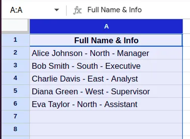
2. Go to the Data tab on the menu bar and choose Split text to columns.

3. Type in the delimiter or separator (the value or character that separates the words you want to split) and preview your result. 

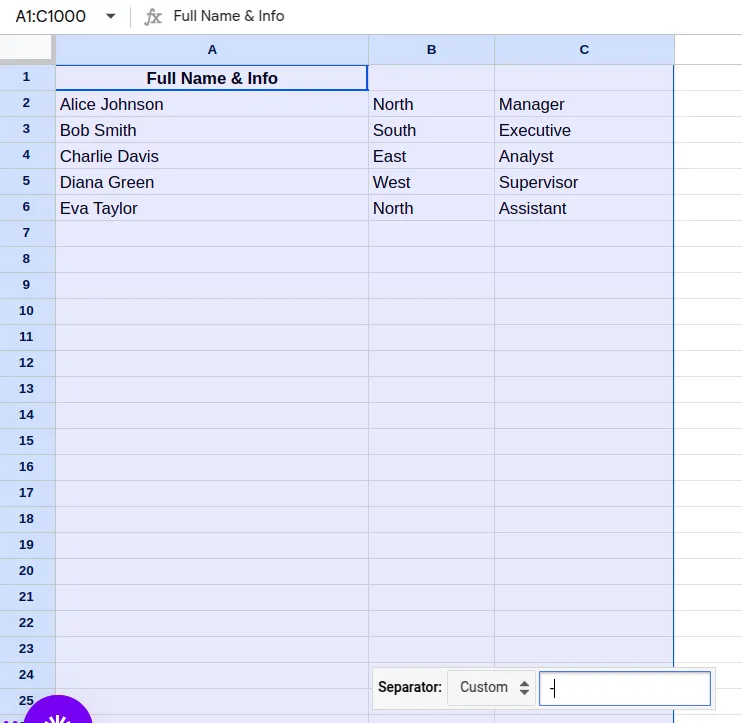
Here, in this example, we had ‘-’, which splits the column based on that delimiter. However, if we have a case where multiple delimiters like ‘-’ and ‘,’ are there, then we need to specify which delimiter to use in the Custom Separator Popup.

10. Extract Prefixes and Suffixes

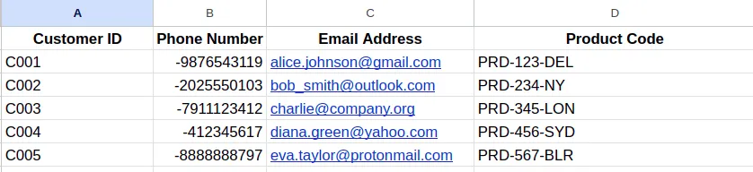
Whenever you are dealing with a variety of data, there might come a situation where you’ll need only part of the data in each cell, such as extracting the area code from a phone number or getting the domain names from email addresses. This is where you can make use of the extraction functions.

Steps to Extract Prefixes and Suffixes

Let’s consider the following dataset

1. To extract the characters from the beginning, we can use the LEFT function. The formula is written as: =LEFT(text, FIND(character, text) – 1)

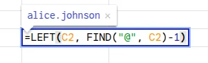
The FIND function here finds the position of @ in the cell, while the LEFT function extracts all the characters before @.

2. To extract characters from the end, we can use the RIGHT function. The formula is written as: =RIGHT(text, LEN(text) – FIND(delimiter, text))

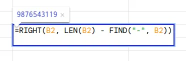
The FIND function here locates the hyphen separating the country code from the number, while the LEN function gives the total length of the string. The formula in its entirety will return the substring after the hyphen.

3. To extract characters from the middle, we can use the MID function. The formula for this function is: =MID(text, FIND(“-“, text) + 1, FIND(“-“, text, FIND(“-“, text) + 1) – FIND(“-“, text) – 1)

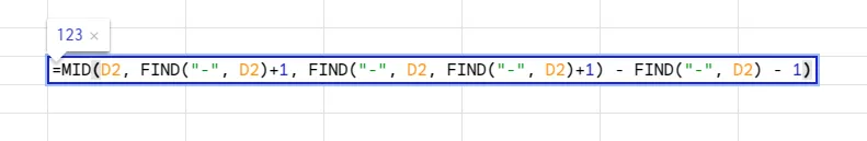
The FIND(“-” D2) function returns the position of the first hyphen. Since we want to extract the info after this, we add the ‘+1’. The FIND(“-”, D2, FIND(“-”, D2) which returns the position of the second hyphen. And since we want to extract text until before this point, we add the ‘-1’. The MID(D2, starts_pos, num_chars) starts extracting just after the first hyphen until the occurrence of the second hyphen.

Conclusion

Clean data is not just a technical necessity but a prerequisite for business intelligence. It lays the foundation that builds and guides million-dollar business decisions. While data cleaning on Excel is a laborious task, I’m sure it’ll be much easier for you now with the methods and formulae discussed in this article.

Mastering the art of how to clean data in Excel takes you to a step much higher than simple data entry workers. It makes you a trusted advisor whose analysis becomes part of the strategy development of your company. Now, to get there, all you need to do is practice on these data cleaning solutions on Excel and make yourself better at it.