Preference Fine-Tuning LFM 2 Using DPO

Liquid Foundation Models (LFM 2) define a new class of small language models designed to deliver strong reasoning and instruction-following capabilities directly on edge devices. Unlike large cloud-centric LLMs, LFM 2 focuses on efficiency, low latency, and memory awareness while still maintaining competitive performance. This design makes it a compelling choice for applications on mobile devices, laptops, and embedded systems where compute and power remain constrained, but reliability is critical.

The core LFM 2 dense models come in sizes of 350M, 700M, 1.2B, and 2.6B parameters, each supporting a 32,768-token context window. This unusually long context for models of this size enables richer reasoning, longer conversations, and better document-level understanding without sacrificing deployability. When paired with DPO, teams can efficiently align LFM 2 to specific behaviors such as tone, safety constraints, domain focus, or instruction-following style. Teams achieve this using simple preference data instead of expensive reinforcement learning pipelines. Because DPO directly fine-tunes the base model without requiring a separate reward model, it keeps training and inference lightweight, making it especially well-suited for edge-focused SLMs where compute, memory, and stability are critical. This combination allows LFM 2 to remain fast and compact while still reflecting user or product-specific preferences.

In this article, we will be covering how we can fine-tune the LFM2-700M model with DPO. So, without any further ado, let’s dive right in.

Understanding LFM 2: Architecture and Performance

Liquid Foundation Models (LFM 2) represent a new generation of hybrid small language models optimized from the ground up for edge and on-device use. The architecture departs from standard transformer-only designs by combining multiplicative gated short-range convolutional layers with a limited number of grouped query attention (GQA) blocks. Researchers identified this hybrid setup using hardware-in-the-loop architecture search under tight latency and memory constraints, enabling efficient utilization of CPUs and other embedded accelerators. By relying on short convolutions for local context and sparse attention for global reasoning, LFM 2 reduces KV-cache requirements and inference cost compared to dense attention-heavy models.

More importantly, LFM 2 achieves significant speed and memory benefits without sacrificing quality. Benchmarks show that LFM 2 models offer up to 2x faster prefill and decode speeds on CPU relative to comparable models, and the entire training pipeline can be 3x more efficient than their predecessors. This performance advantage makes them well-suited for real-time applications where low latency is critical, such as mobile assistants, embedded robotics, real-time translation, and on-device summarization, especially when cloud connectivity is unreliable or undesirable.

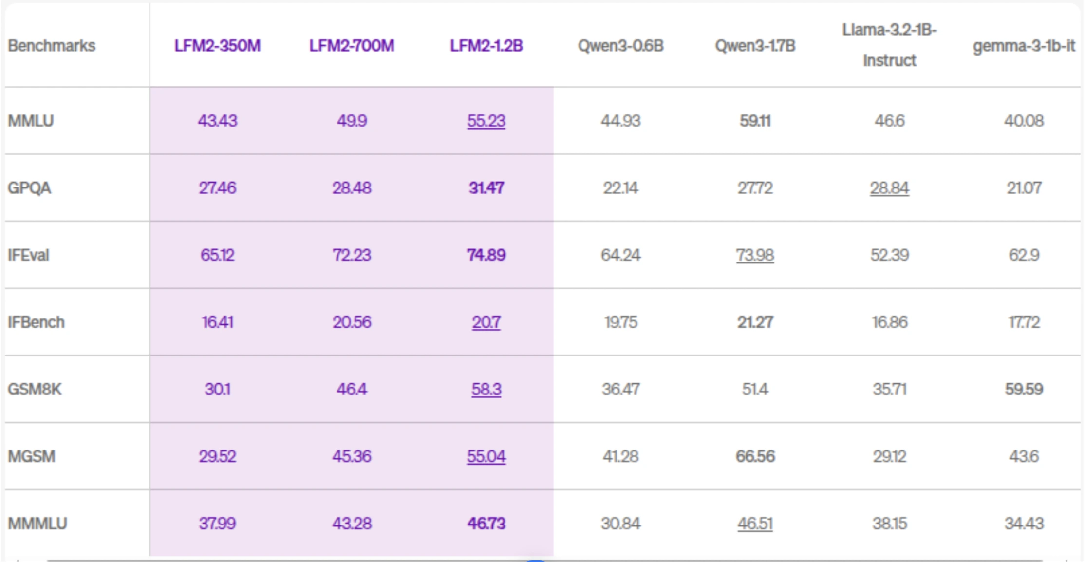
Across standard language benchmarks, LFM 2 models outperform many similarly sized small models in areas such as instruction following, reasoning, multilingual understanding, and mathematics. For example, the flagship 2.6B variant achieves strong results on benchmarks like GSM8K for mathematical reasoning and IFEval for instruction adherence, rivaling models with significantly larger parameter counts. In addition to dense language tasks, the LFM 2 family has been extended into multimodal areas such as vision-language (LFM 2-VL) and audio (LFM 2-Audio) while retaining the core efficiency principles, making the platform flexible for a wide range of AI applications on edge devices.

What is Direct Preference Optimization (DPO)?

Direct Preference Optimization (DPO) is a modern fine-tuning technique designed to align language models with human preferences in a simpler and more stable way than traditional Reinforcement Learning from Human Feedback (RLHF). Instead of training a separate reward model and running complex reinforcement learning loops (like PPO), DPO directly updates the language model using preference data.

In DPO, the model is trained on pairs of responses for the same prompt: one chosen (preferred) and one rejected. These preferences can come from human annotations or even from stronger models acting as judges. A reference model (usually the original base model) is used to stabilize training, and the objective encourages the fine-tuned model to assign higher probability to preferred responses and lower probability to rejected ones. This makes DPO easier to implement, more predictable, and significantly more resource-efficient.

Pros of Direct Preference Optimization

• Simple to implement: No need to train or maintain a separate reward model.
• Stable and predictable: Avoids many of the instabilities associated with PPO-based RLHF.
• Compute-efficient: Directly fine-tunes the model without expensive reinforcement learning loops.
• Well-suited for SLMs: Especially effective when working with smaller models like LFM 2.

Cons of Direct Preference Optimization

• Limited feedback expressiveness: Works primarily with binary (preferred vs. rejected) feedback.
• Less flexible reward design: Cannot encode complex, multi-objective reward functions as easily as full RLHF.

Finetuning LFM 2-700M

So the model we chose to finetune is LFM2-700M. Since this is a small model, it will be effective and will be quicker to fine-tune. Feel free to fine-tune other models of the LFM2 family if you wish.

The dataset we will be using would be mlabonne/orpo-dpo-mix-40k. The mlabonne/orpo-dpo-mix-40k dataset is a preference-based training corpus specifically designed for DPO (Direct Preference Optimization) or ORPO (Off-Policy Reinforcement Preference Optimization) fine-tuning of language models. It’s a mixture dataset that brings together multiple high-quality preference datasets into a single unified collection of labeled preference pairs.

The dataset aggregates samples from several existing preference datasets, each curated for quality and preference information:

• argilla/Capybara-Preferences – high-quality preferred responses (≥5 rating)
• argilla/distilabel-intel-orca-dpo-pairs – preference pairs not in GSM8K with high-scored chosen responses
• argilla/ultrafeedback-binarized-preferences-cleaned – large cleaned preference set
• argilla/distilabel-math-preference-dpo – math-related preference pairs
• M4-ai/prm_dpo_pairs_cleaned – cleaned preference pairs
• jondurbin/truthy-dpo-v0.1 – additional preference sources
• unalignment/toxic-dpo-v0.2 – a smaller set that includes challenging/toxic prompts (often filtered out in practice)

So, let’s proceed with the fine-tuning part now. We use LFM2-700M as our base model since it is a small, efficient language model that fine-tunes quickly and fits comfortably on a T4 GPU.

Step 1: Setting Up the Training Environment

In this step, we install the required libraries for model loading, preference optimization, and parameter-efficient fine-tuning. Using fixed or minimum versions ensures compatibility between Transformers, TRL, and PEFT, especially when running on Google Colab.

!pip install transformers==4.54.0 trl>=0.18.2 peft>=0.15.2 -q

Step 2: Importing Core Libraries and Verifying Versions

Here we import PyTorch, Transformers, and TRL, which form the core of our training pipeline. Printing the version numbers helps ensure reproducibility and avoids subtle issues caused by incompatible library versions.

import torch
import transformers
import trl
import os


print(f"📦 PyTorch version: {torch.__version__}")
print(f"🤗 Transformers version: {transformers.__version__}")
print(f"📊 TRL version: {trl.__version__}")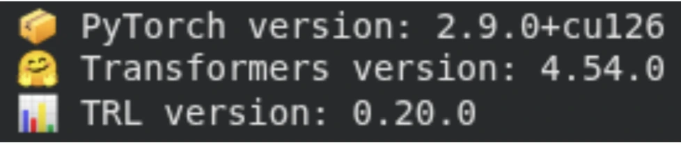

Step 3: Downloading the Tokenizer and Base Model

We load the LFM2-700M tokenizer and model directly from Hugging Face. The tokenizer converts raw text into token IDs, while the model is loaded with automatic device placement using device_map=”auto”, allowing it to efficiently utilize the available GPU. At this stage, we verify the model size, parameter count, and vocabulary size.

from transformers import AutoTokenizer, AutoModelForCausalLM
import torch


model_name = "LiquidAI/LFM2-700M" # <- alter model here to use LiquidAI/LFM2-350M or LFM2-1.2B


print("📚 Loading tokenizer...")
tokenizer = AutoTokenizer.from_pretrained(model_name)


print("🧠 Loading model...")
model = AutoModelForCausalLM.from_pretrained(
   model_name,
   device_map="auto",
   torch_dtype="auto",
)


print("✅ Local model loaded successfully!")
print(f"🔢 Parameters: {model.num_parameters():,}")
print(f"📖 Vocab size: {len(tokenizer)}")
print(f"💾 Model size: ~{model.num_parameters() * 2 / 1e9:.1f} GB (bfloat16)")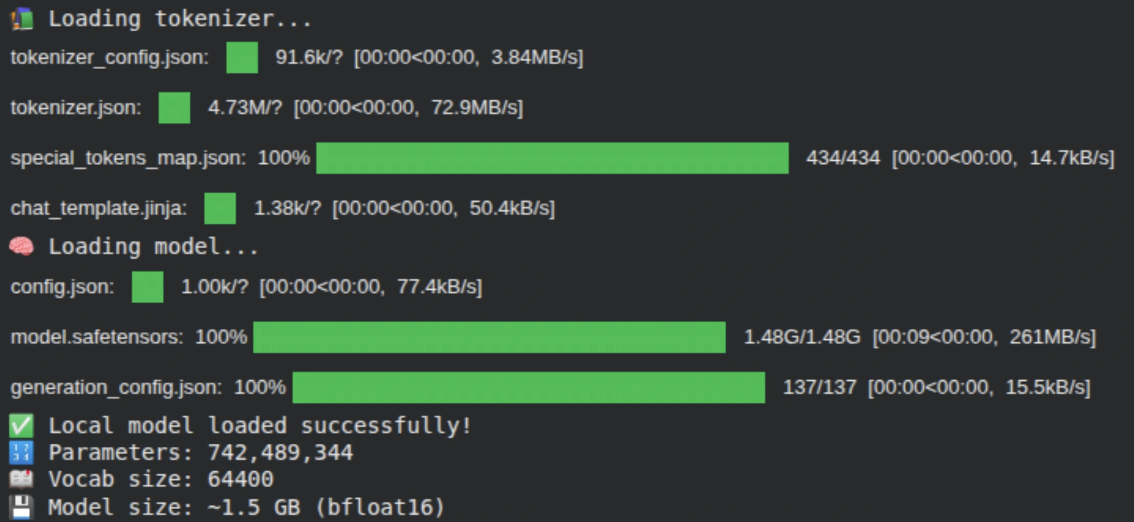

Step 4: Loading and Preparing the Preference Dataset

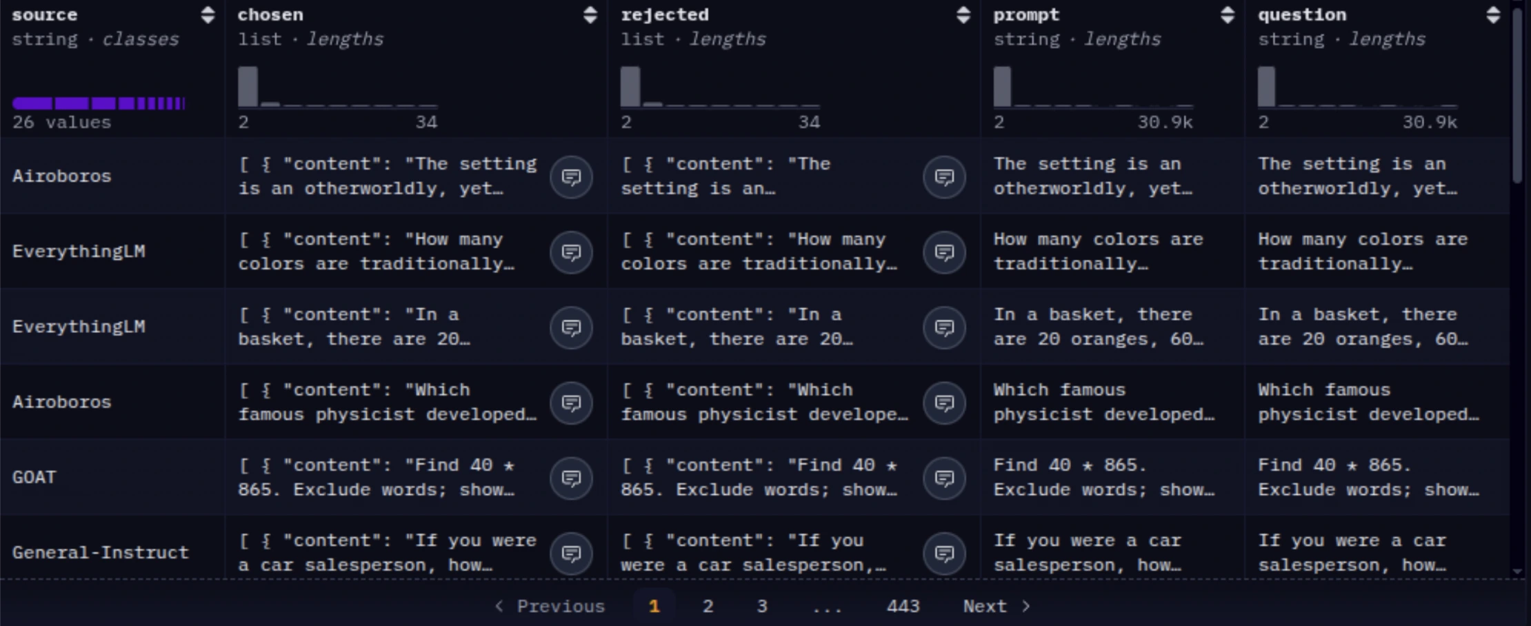
We load the mlabonne/orpo-dpo-mix-40k dataset, which contains preference pairs consisting of a prompt, a preferred response, and a rejected response. To keep training efficient, we use a subset of the data and split it into training and evaluation sets, enabling us to track alignment performance during training.

from datasets import load_dataset


print("📥 Loading DPO dataset...")


dataset_dpo = load_dataset("mlabonne/orpo-dpo-mix-40k", split="train[:2500]")   # number of samples are directly proportional to the training time.
dataset_dpo = dataset_dpo.train_test_split(test_size=0.1, seed=42)
train_dataset_dpo, eval_dataset_dpo = dataset_dpo['train'], dataset_dpo['test']


print("✅ DPO Dataset loaded:")
print(f"   📚 Train samples: {len(train_dataset_dpo)}")
print(f"   🧪 Eval samples: {len(eval_dataset_dpo)}")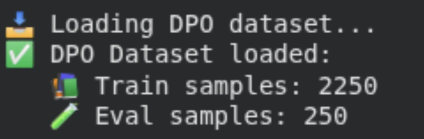

Step 5: Enabling Parameter-Efficient Fine-Tuning with LoRA

Instead of fine-tuning all model parameters, we apply LoRA (Low-Rank Adaptation) using PEFT. We target key components of the LFM2 architecture, including feed-forward (GLU), attention, and convolutional layers. This drastically reduces the number of trainable parameters, making fine-tuning faster and more memory-efficient.

from peft import LoraConfig, get_peft_model, TaskType


GLU_MODULES = ["w1", "w2", "w3"]
MHA_MODULES = ["q_proj", "k_proj", "v_proj", "out_proj"]
CONV_MODULES = ["in_proj", "out_proj"]


lora_config = LoraConfig(
   task_type=TaskType.CAUSAL_LM,
   inference_mode=False,
   r=8,  # <- lower values = fewer parameters
   lora_alpha=16,
   lora_dropout=0.1,
   target_modules=GLU_MODULES + MHA_MODULES + CONV_MODULES,
   bias="none",  # if we define bias then we will more params to train
   modules_to_save=None,
)


lora_model = get_peft_model(model, lora_config)
lora_model.print_trainable_parameters()


print("✅ LoRA configuration applied!")
print(f"🎛️  LoRA rank: {lora_config.r}")
print(f"📊 LoRA alpha: {lora_config.lora_alpha}")
print(f"🎯 Target modules: {lora_config.target_modules}")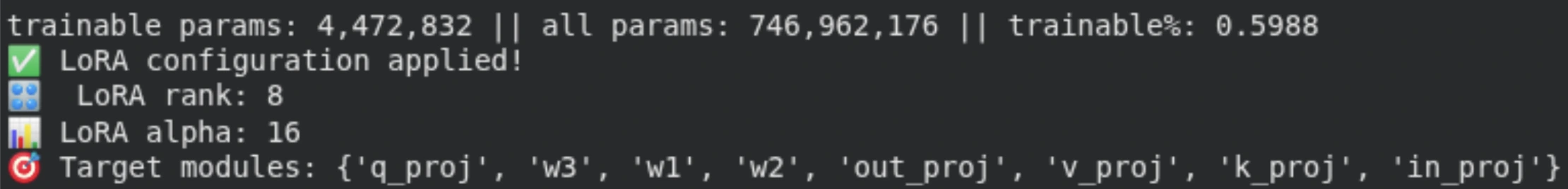

Step 6: Defining the DPO Training Configuration

Here, we specify the Direct Preference Optimization (DPO) training settings, such as learning rate, batch size, gradient accumulation, and evaluation strategy. These parameters gently align the model’s behavior using preference data while maintaining stability on limited GPU hardware.

To lessen your training time, you can use max_steps instead of num_train_epochs, too.

from trl import DPOConfig, DPOTrainer


# DPO Training configuration
dpo_config = DPOConfig(
   output_dir="./lfm2-dpo",
   num_train_epochs=1,           
   per_device_train_batch_size=1,
   learning_rate=1e-6,
   lr_scheduler_type="linear",    # can also use cosine
   gradient_accumulation_steps=4,
   logging_steps=10,
   save_strategy="epoch",
   eval_strategy="epoch",
   bf16=False # <- not all colab GPUs support bf16
)


# Create DPO trainer
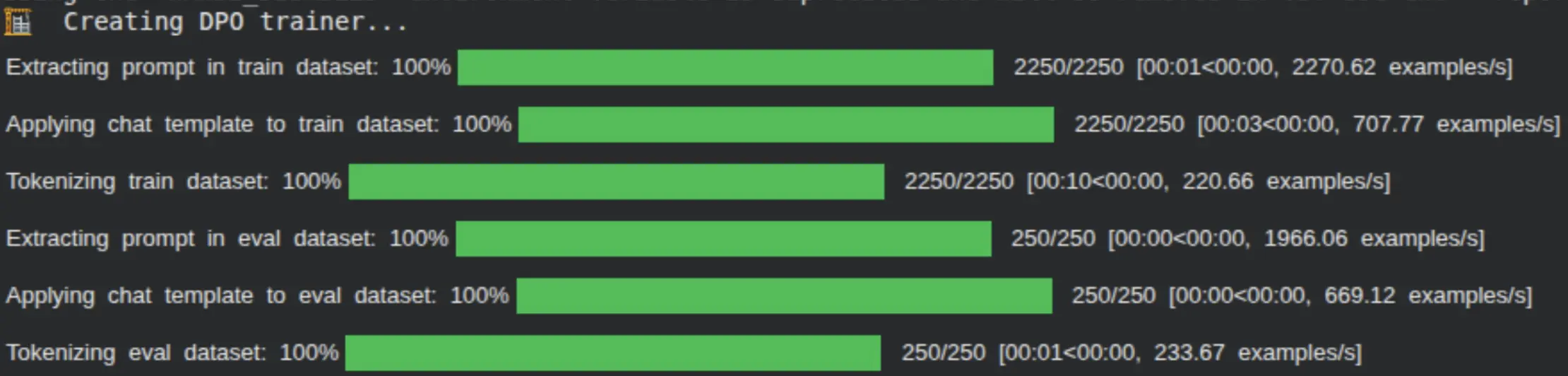
print("🏗️  Creating DPO trainer...")
dpo_trainer = DPOTrainer(
   model=lora_model,
   args=dpo_config,
   train_dataset=train_dataset_dpo,
   eval_dataset=eval_dataset_dpo,
   processing_class=tokenizer,
)

Step 7: Initializing the DPO Trainer

The DPO Trainer brings together the LoRA-wrapped model, tokenizer, datasets, and training configuration. It handles the comparison between chosen and rejected responses and computes the DPO loss that guides the model toward preferred outputs.

# Start DPO training
print("\n🚀 Starting DPO training...")
dpo_trainer.train()


print("🎉 DPO training completed!")


# Save the DPO model
dpo_trainer.save_model()
print(f"💾 DPO model saved to: {dpo_config.output_dir}")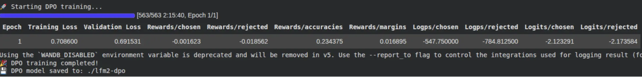

Normally, we will see all our metrics at every 10th step here when the model is being trained.

Step 8: Training the Model with DPO

We now begin DPO training. During this phase, the model learns to assign higher likelihoods to preferred responses and lower likelihoods to rejected ones. Training metrics are logged at regular intervals, allowing us to monitor alignment progress.

print("\n🔄 Merging LoRA weights...")
merged_model = lora_model.merge_and_unload()
merged_model.save_pretrained("./lfm2-lora-merged")
tokenizer.save_pretrained("./lfm2-lora-merged")
print("💾 Merged model saved to: ./lfm2-lora-merged")

Step 9: Merging LoRA Weights and Saving the Final Model

After training, we merge the LoRA adapters back into the base model to create a standalone fine-tuned checkpoint. The merged model and tokenizer are saved locally, making them ready for inference or deployment.

Optionally, we can push the fine-tuned model to the Hugging Face Hub, allowing it to be easily shared, versioned, and reused across projects or deployment environments.

merged_model.push_to_hub("<your-hf-username>/LFM2-700M-DPO-FT")
tokenizer.push_to_hub("<your-hf-username>/LFM2-700M-DPO-FT")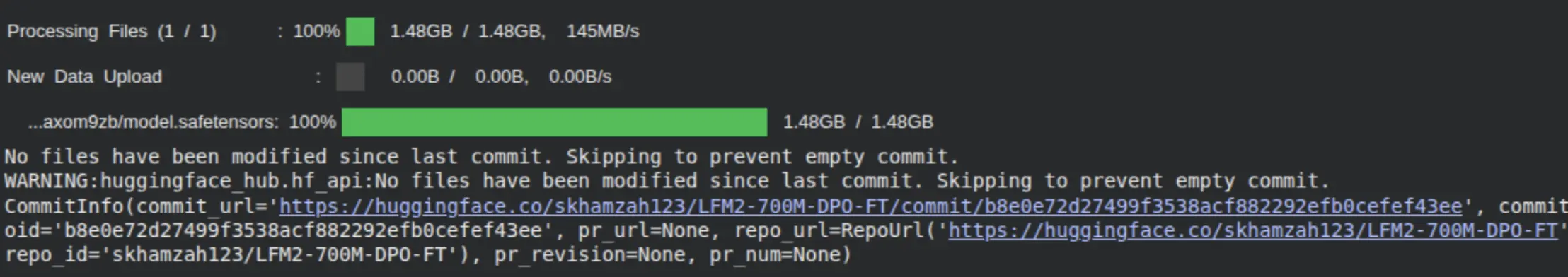

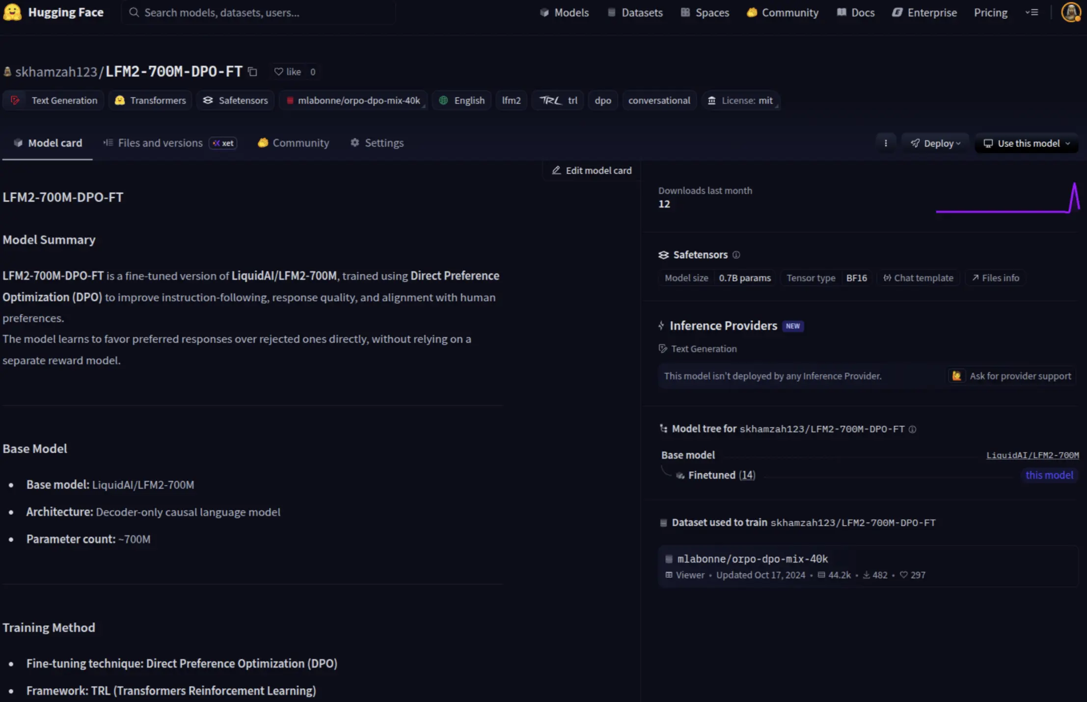
Finally, you would be able to check your model pushed into your Hugging Face account, ready to be used by the public.

Step 10: Running Inference with the Fine-Tuned LFM 2 Model

Now that the model has been fine-tuned and pushed to the Hugging Face Hub, the final step is to load the model and generate responses. This step validates that the Direct Preference Optimization (DPO) training has successfully aligned the model’s behavior and that it can produce high-quality outputs during inference.

We load the fine-tuned checkpoint using AutoModelForCausalLM and AutoTokenizer, ensuring the model runs efficiently by leveraging automatic device placement and reduced-precision weights. We then pass a simple prompt through the tokenizer using the chat template and generate text with controlled sampling parameters, such as temperature and repetition penalty, to encourage coherent and preference-aligned responses.

from transformers import AutoModelForCausalLM, AutoTokenizer


# Load model and tokenizer
model_id = "skhamzah123/LFM2-700M-DPO-FT"
model = AutoModelForCausalLM.from_pretrained(
   model_id,
   device_map="auto",
   torch_dtype="bfloat16",
#    attn_implementation="flash_attention_2" <- uncomment on compatible GPU
)
tokenizer = AutoTokenizer.from_pretrained(model_id)


# Generate answer
prompt = "What is LLMs in simple words?"
input_ids = tokenizer.apply_chat_template(
   [{"role": "user", "content": prompt}],
   add_generation_prompt=True,
   return_tensors="pt",
   tokenize=True,
).to(model.device)


output = model.generate(
   input_ids,
   do_sample=True,
   temperature=0.3,
   min_p=0.15,
   repetition_penalty=1.05,
   max_new_tokens=512,
)


print(tokenizer.decode(output[0], skip_special_tokens=False))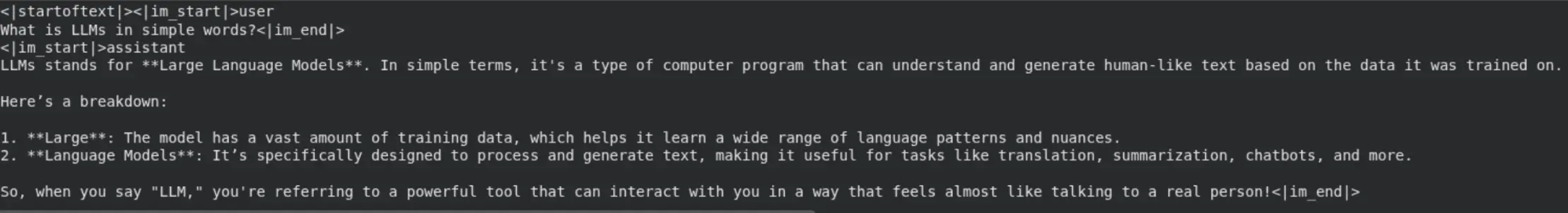

As seen from the output, the model responds in a clear and well-structured manner, demonstrating that the DPO fine-tuning has effectively improved instruction following while maintaining the efficiency and deployability expected from an edge-friendly Small Language Model.

Conclusion

In this blog, we explored how Direct Preference Optimization (DPO) efficiently aligns Liquid Foundation Models (LFM 2) with desired behaviors and preferences. By fine-tuning LFM2-700M, we showed that effective alignment does not require complex reinforcement learning pipelines or large-scale computation. Instead, DPO offers a simpler, more stable, and resource-efficient alternative, making it particularly well-suited for small language models and edge deployments.

Using LoRA-based parameter-efficient fine-tuning, we adapted the model while training only a small subset of parameters, keeping memory usage and training costs low. This workflow allows practitioners to align models on modest hardware while preserving the efficiency and performance characteristics of LFM 2. After training, the result is a standalone checkpoint that is ready for inference, deployment, or sharing.

You guys can also experiment with other LFM 2 variants, including smaller or larger model sizes, and try out different preference datasets tailored to specific domains or use cases. This flexibility makes the approach broadly applicable, whether the goal is instruction tuning, reasoning enhancement, or domain-specific alignment, providing a practical and extensible foundation for building aligned, deployable language models.