Evaluating Deep Learning Models with Custom Loss Functions and Calibration Metrics

Evaluating Deep Learning models is an essential part of model lifecycle management. Whereas traditional models have excelled at providing quick benchmarks for model performance, they often fail to capture the nuanced goals of real-world applications. For instance, a fraud detection system might prioritize minimizing false negatives over false positives, while a medical diagnosis model might value recall more than precision. In such scenarios, relying solely on conventional metrics can lead to suboptimal model behavior. This is where custom loss functions and tailored evaluation metrics come into play.

Conventional Deep Learning Models Evaluation

The conventional measures to evaluate classification include Accuracy, Recall, F1-score, and so on. Cross-entropy loss is the preferred loss function to use for classification. These typical measures of classification evaluate only whether predictions were correct or not, ignoring uncertainty.

A model can have high accuracy but poor probability estimates. Modern deep networks are overconfident and return probabilities of ~0 or ~1 even when they are wrong.

Read more: Conventional model evaluation metrics

The Problem

Guo et al. show that a highly accurate deep model can still be poorly calibrated. Likewise, a model might have a high F1 score but still could be miscalibrated in its uncertainty estimates. Optimizing objective functions like accuracy or log-loss can also produce miscalibrated probabilities, since traditional evaluation metrics do not assess whether the model’s confidence matches reality. For instance, a pneumonia detection AI might output 99.9% probability based on patterns that also occur in harmless conditions, leading to overconfidence. Calibration methods like temperature scaling adjust these scores so they better reflect true likelihoods.

What Are Custom Loss Functions?

A custom loss or objective function is any training loss function (other than standard losses like cross-entropy and MSE) that you invent to express specific goals. You might develop one when a more generic loss does not meet your business requirements. 

For instance, you could use a loss that penalizes false negatives, missed fraud, more than false positives. This lets you handle uneven penalties or goals, like maximizing F1 instead of just accuracy. A loss is simply a smooth mathematical formula that compares predictions with labels, so you can design any formula that closely mimics the metric or cost you want.

Why build a Custom Loss Function?

Sometimes the default loss under-trains on important cases (e.g., rare classes) or doesn’t reflect your utility. Custom losses give you the ability to:

• Align with business logic: e.g., penalize missing a disease 5× more than a false alarm.
• Handle imbalance: downweight the majority class, or focus on the minority.
• Encode domain heuristics: e.g., require predictions to respect monotonicity or ordering.
• Optimize for specific metrics: approximate F1/precision/recall, or domain-specific ROI.

How to Implement a Custom Loss Function?

In this section, we’ll implement a custom loss with PyTorch using the nn.Module function. The following are its key points:

• Differentiability: Make sure the loss function is differentiable for the model outputs.
• Numerical Stability: Use log-sum-exp or stable functions in PyTorch (F.log_softmax, F.cross_entropy, etc.). For example, one can write Focal Loss by using F.cross_entropy (containing softmax and log) in the same way, but then multiplying by (1−𝑝𝑡)𝛾. This method avoids needing to compute the probabilities in a separate softmax, which can underflow.
• Code Example: To demonstrate the idea, here is how one would define a custom Focal Loss in PyTorch:

import torch

import torch.nn as nn

import torch.nn.functional as F

class FocalLoss(nn.Module):

   def __init__(self, gamma=2.0, weight=None):

       super(FocalLoss, self).__init__()

       self.gamma = gamma

       self.weight = weight  # weight tensor for classes (optional)

   def forward(self, logits, targets):

       # Compute standard cross entropy loss per-sample

       ce_loss = F.cross_entropy(logits, targets, weight=self.weight, reduction='none')

       p_t = torch.exp(-ce_loss)          # The model's estimated probability for true class

       loss = ((1 - p_t) ** self.gamma) * ce_loss

       return loss.mean()

Here, γ tunes how much focus we want on the hard examples. The higher γ=more focus, and this implies that weight can handle class imbalance.

We used Focal loss as the loss function as it’s designed to address class imbalance in object detection and other machine learning tasks, particularly when dealing with a large number of easily classified examples, e.g., background in object detection. This makes it suitable for our task. 

Why Model Calibration Matters?

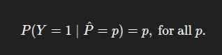
Calibration describes how well predicted probabilities correspond to real-world frequencies. A model is well-calibrated if among all the instances to which it assigns probability p to the positive class, about p fraction are positive. In other words, “confidence = accuracy”. For instance, if a model predicts 0.8 on 100 test cases, we would expect about 80 to be correct. Calibration is important when using probabilities for a decision (e.g., risk scoring; cost-benefit analysis). Formally, that means for a classifier with a probability output 𝑝^, calibration is:

Calibration Errors

Calibration errors fall into two categories:

1. Overconfidence: Means the model’s predicted probabilities are systematically higher than true probabilities (e.g., predicts 90%, but is right 80% of the time). Deep neural networks tend to be overconfident, especially when overparameterized. Overconfident models can be dangerous; they often make strong predictions and can mislead us when misclassifying.
2. Underconfidence: Underconfidence is less common in deep nets. This is the opposite of overconfidence, when the model’s confidence is too low (e.g., predicts 60%, but is right 80% of the time). While underconfidence typically places the model in a safer position when predicting, it may look unsure and thus less useful.

In practice, modern DNNs are typically overconfident. Guo et al. found that newer deep nets with batch norm, deeper layers, etc., had spiky posterior distributions with very high probability on one class, even while misclassifying. When we make these miscalibrations, it is critical to realize them so we can make reliable predictions.

Metrics for Calibration

• Reliability Diagram: Calibration Curve Commonly called a reliability diagram, this also casts the predicted successes into bins based on the prediction’s confidence score. For each bin, it plots the proportion of positives (y-axis) vs. the mean predicted probability on the x-axis.

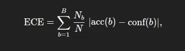
• Expected Calibration Error (ECE): It summarizes the absolute difference between accuracy and confidence, weighted by the size of the bin. Formally, where acc(b) and conf(b) are the accuracy and mean confidence in bin size. As a reminder, lower values of ECE are better (0=perfectly calibrated). ECE is a measure of average miscalibration. 

• Maximum Calibration Error (MCE): The largest gap over all bins:

• Brier Score: Brier score is the mean squared error between the predicted probability and the actual outcome, which is either 0 or 1. It is a proper scoring rule and captures both calibration and accuracy. However, a smaller Brier score does not mean the predictions are well calibrated. It combines calibration and discrimination.

Read more: Calibration of Machine Learning Models

Case Study using PyTorch

Here, we’ll use the BigMart Sales dataset to demonstrate how the custom loss functions and the calibration matrices help in predicting the target column, OutletSales.

We change the continuous OutletSales to a binary High vs Low class by thresholding at the median. We then fit a simple classifier in PyTorch using features such as product visibility, and then apply custom loss and calibration. 

Key steps

Data Preparation and Preprocessing: In this part, we’ll import the libraries, load the data, and most importantly, do the data preprocessing steps. Like missing value handling, making the categorical column uniform (‘low fat’, ‘Low Fat’, and lf all are the same so they’ll become “Low Fat”), making a threshold for the target variable, performing OHE (One-hot encoding) on categorical variables, and splitting the features.

import os
import random
import numpy as np
import pandas as pd
import matplotlib.pyplot as plt

import torch
import torch.nn as nn
import torch.nn.functional as F
from torch.utils.data import TensorDataset, DataLoader, random_split

from sklearn.preprocessing import StandardScaler
from sklearn.model_selection import train_test_split
from sklearn.metrics import classification_report, confusion_matrix
from sklearn.utils.class_weight import compute_class_weight


SEED = 42
random.seed(SEED)
np.random.seed(SEED)
torch.manual_seed(SEED)

if torch.cuda.is_available():
    torch.cuda.manual_seed_all(SEED)

device = torch.device('cuda' if torch.cuda.is_available() else 'cpu')
print('Device:', device)

# ----- missing-value handling -----
df['Weight'].fillna(df['Weight'].mean(), inplace=True)
df['OutletSize'].fillna(df['OutletSize'].mode()[0], inplace=True)

# ----- categorical cleaning -----
df['FatContent'].replace(
    {'low fat': 'Low Fat', 'LF': 'Low Fat', 'reg': 'Regular'},
    inplace=True
)

# ----- classification target -----
threshold = df['OutletSales'].median()
df['SalesCategory'] = (df['OutletSales'] > threshold).astype(int)

# ----- one-hot encode categoricals -----
cat_cols = [
    'FatContent', 'ProductType', 'OutletID',
    'OutletSize', 'LocationType', 'OutletType'
]
df = pd.get_dummies(df, columns=cat_cols, drop_first=True)

# ----- split features / labels -----
X = df.drop(['ProductID', 'OutletSales', 'SalesCategory'], axis=1).values
y = df['SalesCategory'].values

X_train, X_test, y_train, y_test = train_test_split(
    X, y, test_size=0.2, random_state=SEED, stratify=y
)

scaler = StandardScaler()
X_train = scaler.fit_transform(X_train)
X_test = scaler.transform(X_test)

# create torch tensors
X_train_t = torch.tensor(X_train, dtype=torch.float32)
y_train_t = torch.tensor(y_train, dtype=torch.long)
X_test_t = torch.tensor(X_test, dtype=torch.float32)
y_test_t = torch.tensor(y_test, dtype=torch.long)

# split train into train/val (80/20 of original train)
val_frac = 0.2
val_size = int(len(X_train_t) * val_frac)
train_size = len(X_train_t) - val_size

train_ds, val_ds = random_split(
    TensorDataset(X_train_t, y_train_t),
    [train_size, val_size],
    generator=torch.Generator().manual_seed(SEED)
)

train_loader = DataLoader(
    train_ds, batch_size=64, shuffle=True, drop_last=True
)
val_loader = DataLoader(
    val_ds, batch_size=256, shuffle=False
)

Custom Loss: In the 2nd step, first, we’ll create a custom SalesClassifier. Consider that we apply Focal Loss to place more emphasis on the minority class. Then, we’ll refit the model to maximize Focal Loss instead of Cross Entropy Loss. In many cases, the Focal Loss increases recall on the minor class but may decrease raw accuracy. After that, we’ll train our sales classifier with the help of the custom SoftF1Loss over 100 epochs and save the best model as best_model.pt

class SalesClassifier(nn.Module):

   def __init__(self, input_dim):

       super().__init__()

       self.net = nn.Sequential(

           nn.Linear(input_dim, 128),

           nn.BatchNorm1d(128),

           nn.ReLU(inplace=True),

           nn.Dropout(0.5),

           nn.Linear(128, 64),

           nn.ReLU(inplace=True),

           nn.Dropout(0.25),

           nn.Linear(64, 2)          # logits for 2 classes

       )

   def forward(self, x):

       return self.net(x)

# class-weighted CrossEntropy to fight imbalance

class_weights = compute_class_weight('balanced',

                                    classes=np.unique(y_train),

                                    y=y_train)

class_weights = torch.tensor(class_weights, dtype=torch.float32,

                            device=device)

ce_loss = nn.CrossEntropyLoss(weight=class_weights)

Here, we’ll be using a custom loss function named SoftF1Loss. So here the SoftF1Loss is a custom loss function that directly optimizes for the F1-score in a differentiable way, making it suitable for gradient-based training. Instead of using hard 0/1 predictions, it works with soft probabilities from the model’s output (torch.softmax), so the loss changes smoothly as predictions change. It calculates the soft true positives (TP), false positives (FP), and false negatives (FN) using these probabilities and the true labels, then computes soft precision and recall. From these, it derives a “soft” F1-score and returns 1 – F1 so that minimizing the loss will maximize the F1-score. This is especially useful when dealing with imbalanced datasets where accuracy isn’t a good measure of performance.

# Differentiable Custom Loss Function Soft-F1 loss

class SoftF1Loss(nn.Module):

   def forward(self, logits, labels):

       probs = torch.softmax(logits, dim=1)[:, 1]   # positive-class prob

       labels = labels.float()

       tp = (probs * labels).sum()

       fp = (probs * (1 - labels)).sum()

       fn = ((1 - probs) * labels).sum()

       precision = tp / (tp + fp + 1e-7)

       recall    = tp / (tp + fn + 1e-7)

       f1 = 2 * precision * recall / (precision + recall + 1e-7)

       return 1 - f1

f1_loss = SoftF1Loss()

def total_loss(logits, targets, alpha=0.5):

   return alpha * ce_loss(logits, targets) + (1 - alpha) * f1_loss(logits, targets)

model = SalesClassifier(X_train.shape[1]).to(device)

optimizer = torch.optim.Adam(model.parameters(), lr=1e-3)

best_val = float('inf'); patience=10; patience_cnt=0

for epoch in range(1, 101):

   model.train()

   train_losses = []

   for xb, yb in train_loader:

       xb, yb = xb.to(device), yb.to(device)

       optimizer.zero_grad()

       logits = model(xb)

       loss = total_loss(logits, yb)

       loss.backward()

       optimizer.step()

       train_losses.append(loss.item())

   # ----- validation -----

   model.eval()

   with torch.no_grad():

       val_losses = []

       for xb, yb in val_loader:

           xb, yb = xb.to(device), yb.to(device)

           val_losses.append(total_loss(model(xb), yb).item())

       val_loss = np.mean(val_losses)

   if epoch % 10 == 0:

       print(f'Epoch {epoch:3d} | TrainLoss {np.mean(train_losses):.4f}'

             f' | ValLoss {val_loss:.4f}')

   # ----- early stopping -----

   if val_loss < best_val - 1e-4:

       best_val = val_loss

       patience_cnt = 0

       torch.save(model.state_dict(), 'best_model.pt')

   else:

       patience_cnt += 1

       if patience_cnt >= patience:

           print('Early stopping!')

           break

# load best weights

model.load_state_dict(torch.load('best_model.pt'))

Calibration Before/After: In this flow, we may have found that the ECE for the baseline model was high, indicating the model was overconfident. So the  Expected Calibration Error (ECE) for the baseline model may be high/low, indicating the model was overconfident/underconfident. 

We can now calibrate the model using temperature scaling and then repeat the process to calculate a new ECE and plot a new reliability curve. We will see that the reliability curve may move closer to the diagonal after temperature scaling occurs.

class ModelWithTemperature(nn.Module):

   def __init__(self, model):

       super().__init__()

       self.model = model

       self.temperature = nn.Parameter(torch.ones(1) * 1.5)

   def forward(self, x):

       logits = self.model(x)

       return logits / self.temperature

model_ts = ModelWithTemperature(model).to(device)

optim_ts = torch.optim.LBFGS([model_ts.temperature], lr=0.01, max_iter=50)

def _nll():

   optim_ts.zero_grad()

   logits = model_ts(X_val := X_test_t.to(device))   # use test set to fit T

   loss = ce_loss(logits, y_test_t.to(device))

   loss.backward()

   return loss

optim_ts.step(_nll)

print('Optimal temperature:', model_ts.temperature.item())

Optimal temperature: 1.585491418838501

Visualization: In this section, we’ll be plotting reliability diagrams “before” and “after” calibration. The diagrams are a visual representation of the improved alignment.

@torch.no_grad()

def get_probs(mdl, X):

   mdl.eval()

   logits = mdl(X.to(device))

   return F.softmax(logits, dim=1).cpu()

def ece(probs, labels, n_bins=10):

   conf, preds = probs.max(1)

   accs = preds.eq(labels)

   bins = torch.linspace(0,1,n_bins+1)

   ece_val = torch.zeros(1)

   for lo, hi in zip(bins[:-1], bins[1:]):

       mask = (conf>lo) & (conf<=hi)

       if mask.any():

           ece_val += torch.abs(accs[mask].float().mean() - conf[mask].mean()) \

                      * mask.float().mean()

   return ece_val.item()

def plot_reliability(ax, probs, labels, n_bins=10, label='Model'):

   conf, preds = probs.max(1)

   accs = preds.eq(labels)

   bins = torch.linspace(0,1,n_bins+1)

   bin_acc, bin_conf = [], []

   for i in range(n_bins):

       mask = (conf>bins[i]) & (conf<=bins[i+1])

       if mask.any():

           bin_acc.append(accs[mask].float().mean().item())

           bin_conf.append(conf[mask].mean().item())

   ax.plot(bin_conf, bin_acc, marker='o', label=label)

   ax.plot([0,1],[0,1],'--',color='orange')

   ax.set_xlabel('Confidence'); ax.set_ylabel('Accuracy')

   ax.set_title('Reliability Diagram'); ax.grid(); ax.legend()

probs_before = get_probs(model   , X_test_t)

probs_after  = get_probs(model_ts, X_test_t)

print('\nClassification report (calibrated logits):')

print(classification_report(y_test, probs_after.argmax(1)))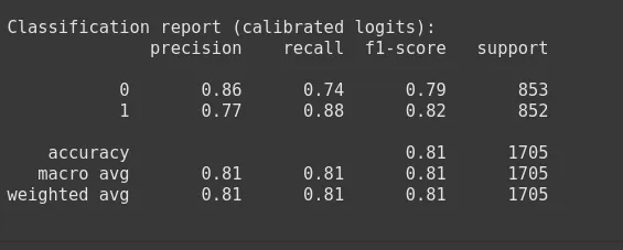

print('ECE before T-scaling :', ece(probs_before, y_test_t))

print('ECE after  T-scaling :', ece(probs_after , y_test_t))

#----------------------------------------

# ECE before T-scaling : 0.05823298543691635

# ECE after  T-scaling : 0.02461853437125683

# ----------------------------------------------

# reliability plot

fig, ax = plt.subplots(figsize=(6,5))

plot_reliability(ax, probs_before, y_test_t, label='Before T-Scaling')

plot_reliability(ax, probs_after , y_test_t, label='After  T-Scaling')

plt.show()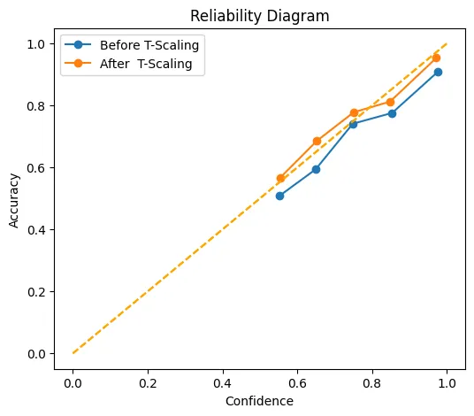

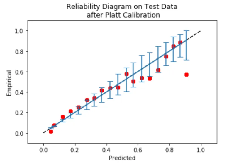
This chart shows how well the confidence score matches/aligns with the actual values, both before (blue) and after (orange) temperature scaling. The x-axis reflects their mean stated confidence, while the y-axis reflects how frequently those predictions were scored properly. The dotted diagonal line represents perfect calibration points that coincide with this line, representing.

For example, predictions that are scored with 70% confidence are correctly scored 70% of the time. After scaling, the orange line hugs this diagonal line more closely than the blue line does. Especially in the ‘middle’ of the confidence space between 0.6 and 0.9 confidence, and almost meets the ideal point at (1.0, 1.0). In other words, temperature scaling has the potential to reduce the model’s proclivity toward over- or under-confidence so that its point estimates of the probability are considerably more accurate.

Check the complete notebook here.

Conclusion

In real-world AI applications, validity and calibration are equally important. A model may have high validity, but if the model’s confidence is not accurate, then there is little value in having higher validity. Therefore, developing custom loss functions particular to your problem statement during the training can fit our true objectives, and we evaluate calibration so we can interpret predictive probabilities appropriately. 

Therefore full evaluation strategy considers both: we first allow the custom losses to fully optimize the model for the task, and then we intentionally calibrate and validate the probability outputs. Now we can create a decision-support tool, where a “90% confidence” really is “90% likely,” which is critical for any real-world implementation.

Read more: Top 7 Loss functions for Regression models

Frequently Asked Questions