This article was published as a part of the Data Science Blogathon.
Introduction

This article will help you get hands-on with python and introduces the preliminary data analysis techniques to get to know your data better.
Often, day to day work of data scientists involve learning multiple algorithms and finding the ML apt solution for varied business problems. They also need to keep themselves updated with the programming language to implement their solution.
Hence, I am writing this article with the intent to cover the basics of the much sought-after programming language these days — python.
I will use ‘german credit risk’ data and will illustrate the analysis with the help of examples to get easy hands-on with this programming tool.
So, let’s get started.
Imports
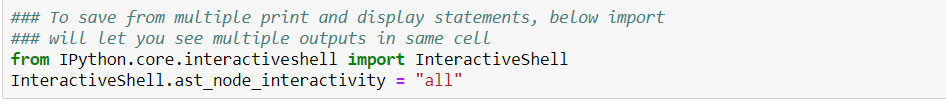
Let’s make all necessary imports:
When we have to type multiple print statements to see the corresponding outputs in a cell in the Jupyter notebook. Below import will let you see multiple outputs in the same cell and saves from multiple prints and display statements.
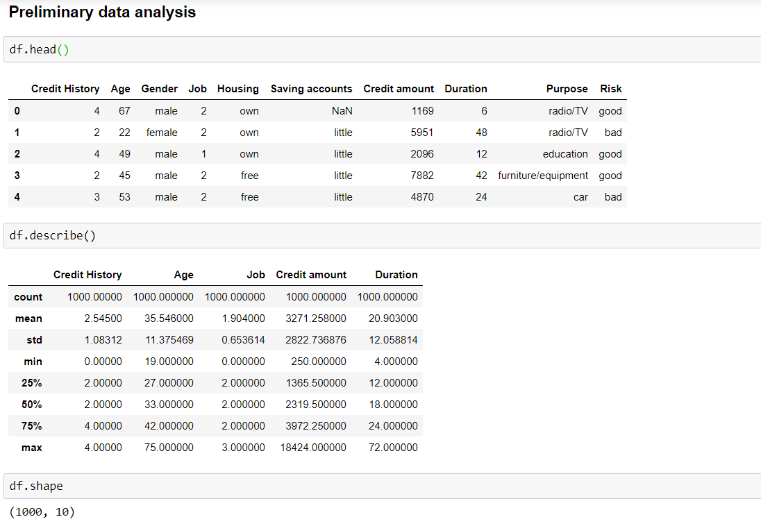
Data exploration:
Let’s start with basic data exploration to check the summary of the data, how it looks like, the size of data, etc.
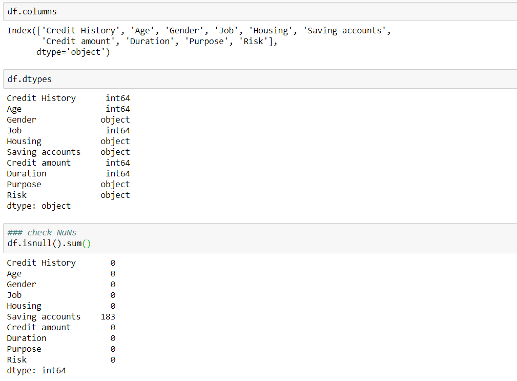
The next important step is to check the data types of each of the columns and see how many null values exist in the data.
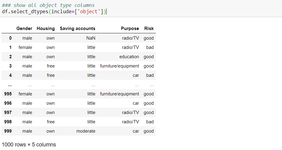
Once we know different data types, we might want to check the data for each category. e.g., the below code lets you see the data frame filtered for only the ‘object’ type:
In order to get all the categorical column names to perform encoding techniques, you can write ‘.columns’ like below:
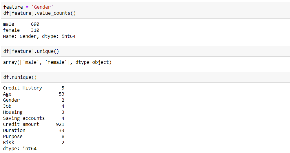
It is important to understand the data feature by feature, e.g. what different range of values each feature takes and count of it:
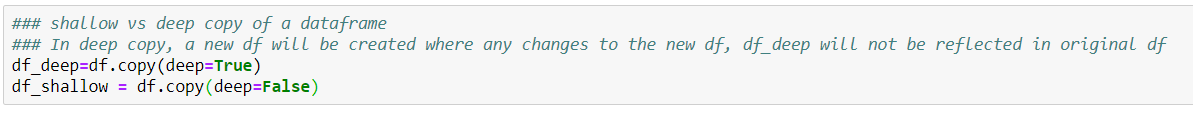
When we want to make some transformation on the original dataframe, we make a copy of it. Making a deep copy of a dataframe prevents the changes made in the new dataframe to get reflected in the original dataframe.
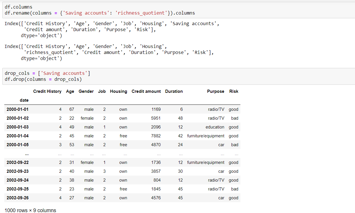
Columns — rename and drop columns
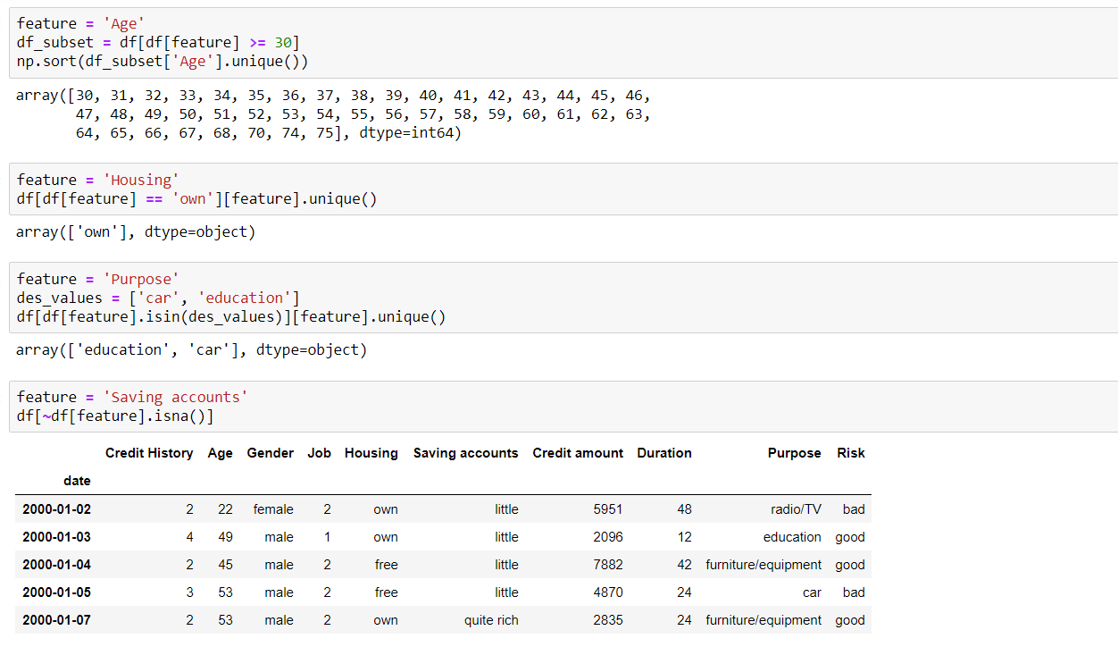
Filtering a dataframe
Great, so we have seen basic techniques of how to use python to get a better understanding of our data.
Datetime:
Next, we will learn how to handle DateTime features.
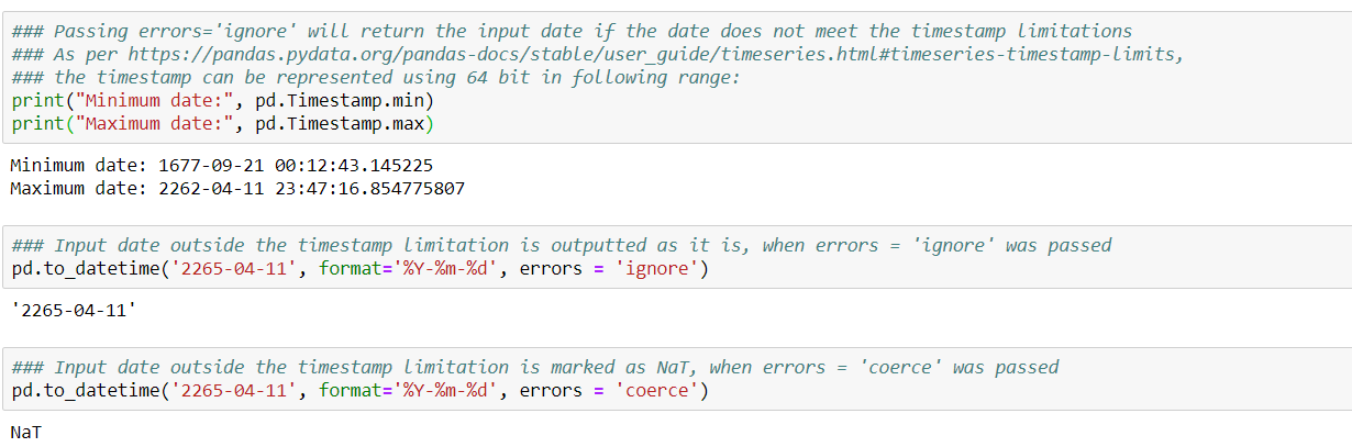
Pandas follow timestamp limitations and can represent timestamp only if it is within a certain range using 64 bits, as shown below. Thus, it will either return the input date as it is, or it will return NaT on the basis of what value we pass for input parameter ‘errors’.
dateutil.parser:
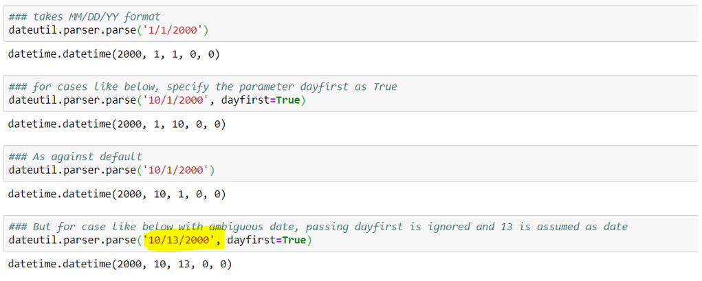
Date as the string is passed as an input to get the datetime format. If dayfirst=True is passed in input, it will assume the DD/MM/YY format.
One good thing is if we pass the date string where the second number corresponding to month is greater than 12 along with dayfirst = True, it will automatically infer that month can not be greater than 12, hence the first number is marked as a month, keeping the second number as day.
It is highlighted below:
strptime and strftime:
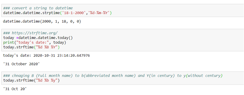
String date can be converted to datetime using strptime. Different formats are specified for the input date. More can be learned about the formats from here.
Conversely, strftime is used to convert datetime to string date.
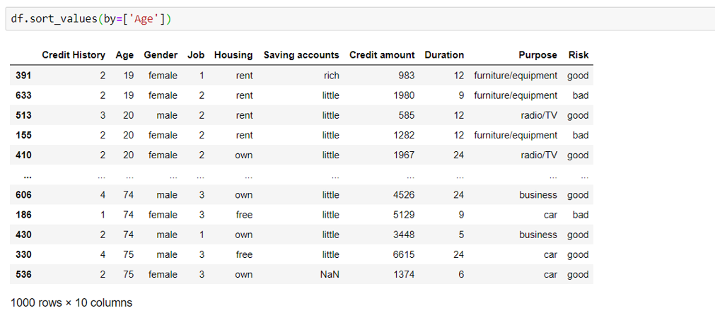
Sorting
The dataframe is sorted by the feature ‘Age’ below:
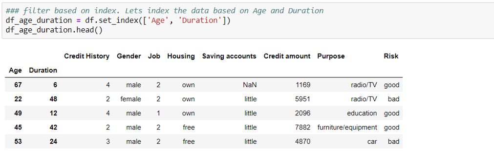
Setting Index
The dataframe can be indexed by one or more columns as below:
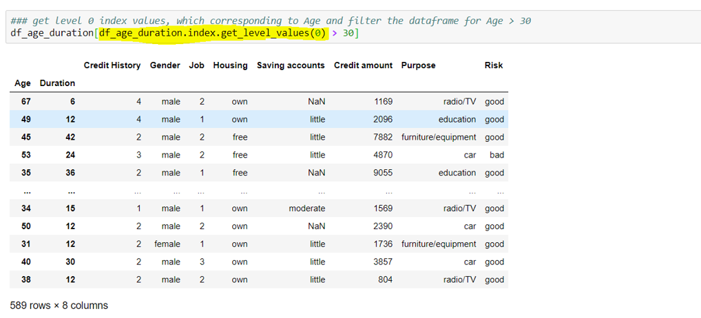
How to filter the Indexed dataframe?
E.g. I have filtered the dataframe by filtering on ‘Age’ index (accessed via ‘0’ level) greater than 30, as highlighted below:
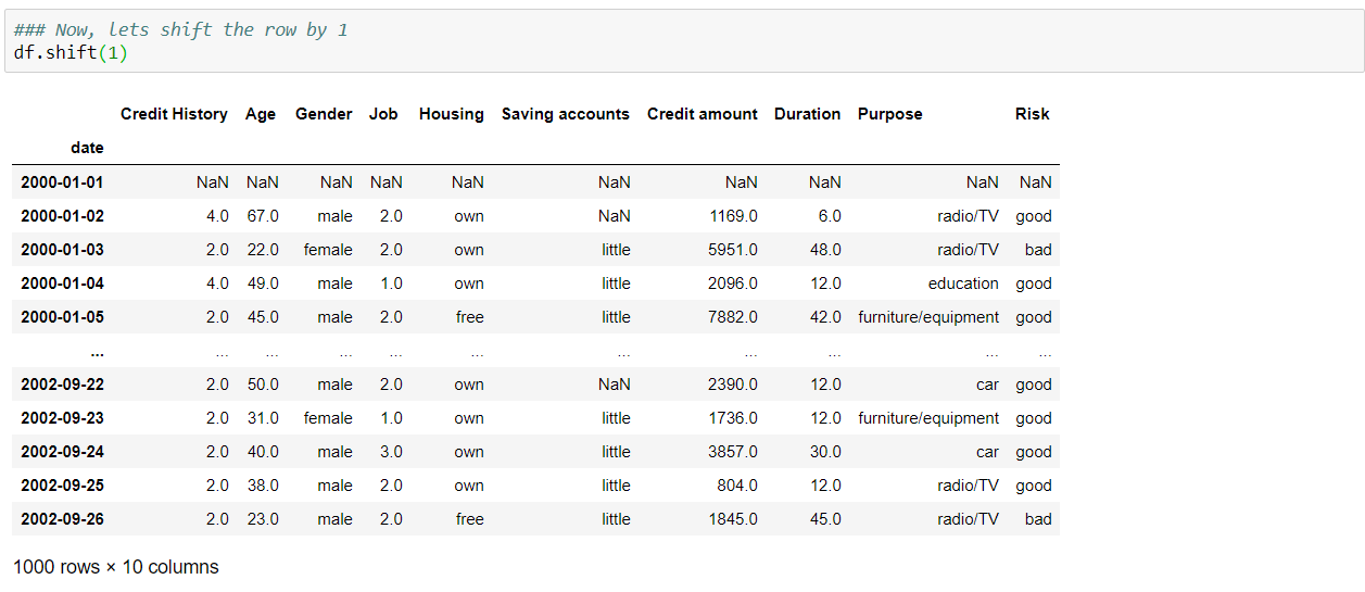
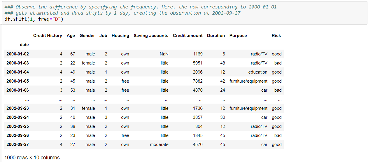
Shifting the dataframe indexed by date:
Dropping NaNs:
Null values can be dropped from the rows by specifying axis=0 and from the columns by specifying axis=1.
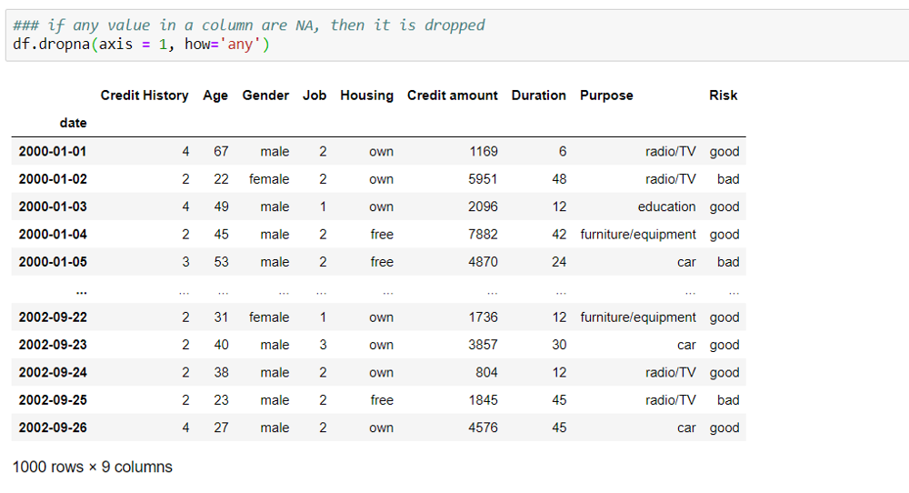
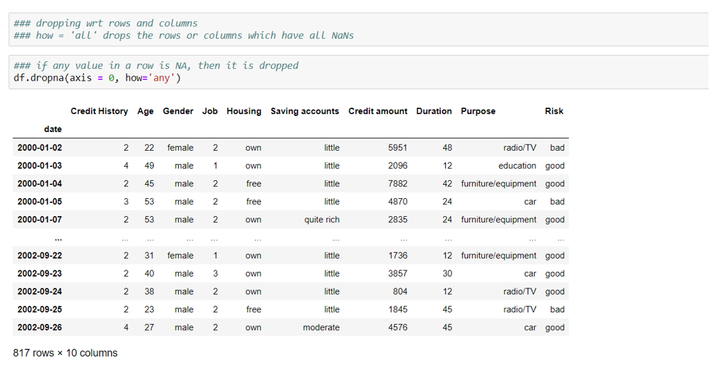
how = ‘any’ and ‘all’ is used to drop the rows/columns where any value is NaN vs the ones where all values are NaNs
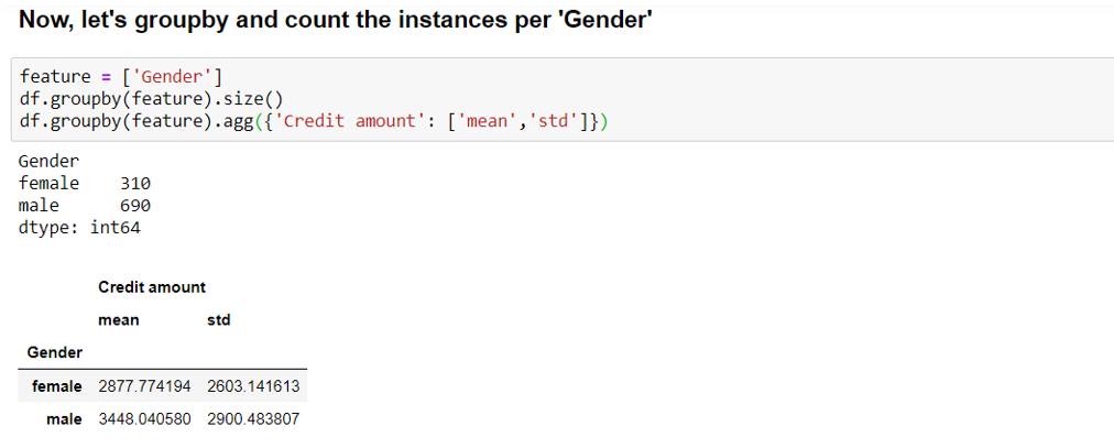
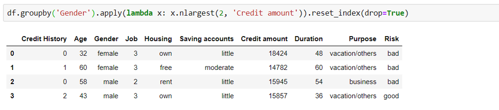
Groupby
The top 2 observations based on ‘Credit amount’ per ‘Gender’ is shown below:
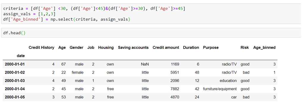
np.select
It is used when multiple conditions are specified, e.g. binning the ‘Age’ variable as per the below criteria, we get the new feature ‘Age_binned’:
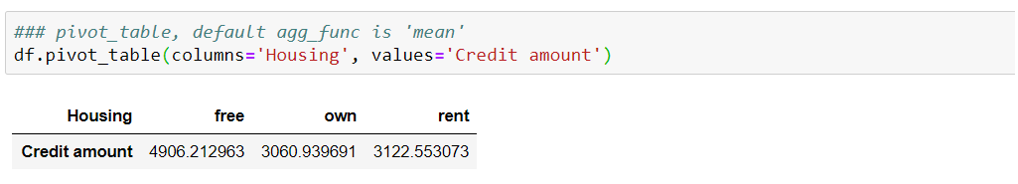
pivot_table
The code can be found in this Jupyter notebook.
Thanks for reading this guide to basic data exploration !!!


