Getting Started with Graph Neural Networks

This article was published as a part of the Data Science Blogathon

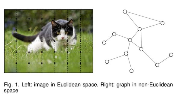
Table of contents

1. The motivation behind Graph Neural Networks

2. GNN Algorithm

3. GNN implementation on Karate network

4. Applications of GNN

5. Challenges of GNN

6. Study papers on GNN

The motivation behind Graph Neural Networks

Graphs are receiving a lot of attention nowadays due to their ability to represent the real world in a fashion that can be analyzed objectively. Graphs can be used to represent a lot of real-world datasets such as social networks, molecular structures, geographical maps, weblink data, natural science, protein-protein interaction networks, knowledge graphs, etc. Also, non-structured data such as images and text can be modelled in the form of graphs. Graphs are data structures that model a set of objects(nodes) and their relationships (edges).

As a unique non-Euclidean data structure for machine learning, graph analysis focuses on tasks like node classification, graph classification, link prediction, graph clustering, and graph visualization. Graph neural networks (GNNs) are deep learning-based methods that operate on graph domains. Due to its good performance in real-world problems involving non-Euclidean space, Graph Neural Networks has become a widely applied graph analysis method recently.

Image 1

Graph Neural Networks Algorithm

A node can be represented by its features and the neighbouring nodes in the graph. The target of GNN is to learn a state embedding, which encodes the information of the neighborhood, for each node. The state embedding is used to produce an output, such as the distribution of the predicted node label.

GNNs is a combination of an information diffusion mechanism and neural networks, representing a set of transition functions and a set of output functions. The information diffusion mechanism is represented by nodes in which their states are updated and information is exchanged by passing “messages” to their neighbouring nodes until they reach a stable equilibrium. The transition function takes the features of each node, the edge features of each node, the neighbouring nodes’ state, and the neighbouring nodes’ features as input and the output is the nodes’ new state.

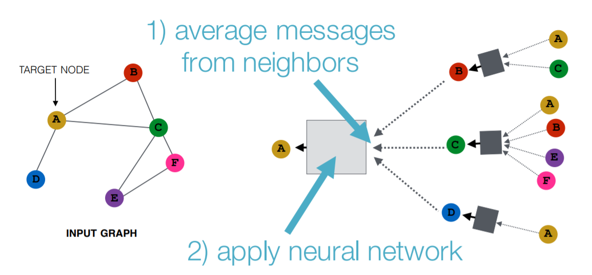
Image 2

Graph Neural Networks implementation on Karate network

In this section, let’s see how we can apply GNN to the Karate network, one of the simple graph networks.

1. Karate network data background:

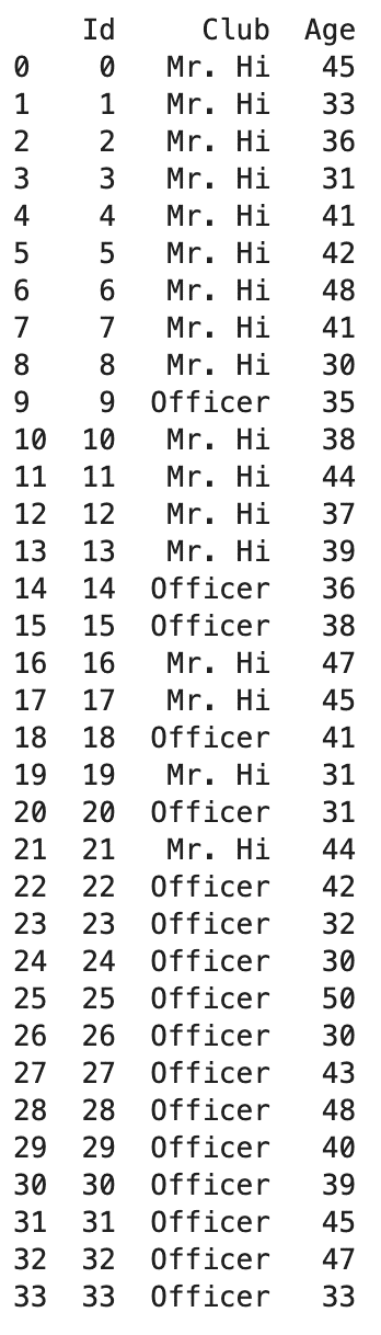
Two 34×34 matrices – 1. ZACHE symmetric, binary

2. ZACHC symmetric, valued.

These are data collected from the members of a university karate club by Wayne Zachary. The ZACHE matrix represents the presence or absence of ties among the members of the club; the ZACHC matrix indicates the relative strength of the associations (number of situations in and outside the club in which interactions occurred).

Zachary (1977) used this data and an information flow model of network conflict resolution to explain the split-up of this group following disputes among the members.

2. Data used:

This data can be converted to 2 CSV files:

1. The nodes.csv stores every club member and their attributes. 34 club members are represented by “Id” from 0 to 33. The club in which they lie – Mr Hi(Node id 0) or Mr Officer(Node id 1) is represented by the “Club” column.
2. The edges.csv stores the pair-wise interactions between two club members. Weightage is given to these interactions between node ids represented by the ‘Weight’ feature.

Nodes.csv – Self Project

Edges.csv – Self Project

3. Using DGL library for graph representation:

We then construct a graph where each node is a club member and each edge represents their interactions. In DGL, nodes are consecutive integers starting from zero. Thus, when preparing the data, it is important to re-label or re-shuffle the row order so that the first row corresponding to the first nodes, so on and so forth.

In this example, we have already prepared the data in the correct order, so we can create the graph by the ‘Src’ and ‘Dst’ columns from the edges.csv table.

Code for loading dgl graph :

import dgl
src = edges_data['Src'].to_numpy()
dst = edges_data['Dst'].to_numpy()
# Create a DGL graph from a pair of numpy arrays
g = dgl.graph((src, dst))

For visualization purposes, we can convert dgl graph to network graph as :

import networkx as nx
# Since the actual graph is undirected, we convert it for visualization purpose.
nx_g = g.to_networkx().to_undirected()
# Kamada-Kawaii layout usually looks pretty for arbitrary graphs
pos = nx.kamada_kawai_layout(nx_g)
nx.draw(nx_g,pos, with_labels=True)

DGL graph network – Self project

4. GNN Model Training on Karate network:

Adding club feature to dgl graph as :

# The "Club" column represents which community does each node belong to.
# The values are of string type, so we must convert it to either categorical
# integer values or one-hot encoding.
club = nodes_data['Club'].to_list()
# Convert to categorical integer values with 0 for 'Mr. Hi', 1 for 'Officer'.
club = torch.tensor([c == 'Officer' for c in club]).long()
# We can also convert it to one-hot encoding.
club_onehot = F.one_hot(club)
print(club_onehot)
# Use `g.ndata` like a normal dictionary
g.ndata.update({'club' : club, 'club_onehot' : club_onehot})

Updating edge features to dgl graph as :

# Get edge features from the DataFrame and feed it to graph.
edge_weight = torch.tensor(edges_data['Weight'].to_numpy())
# Similarly, use `g.edata` for getting/setting edge features.
g.edata['weight'] = edge_weight

Updating Node embeddings:

node_embed = nn.Embedding(g.number_of_nodes(), 5)  # Every node has an embedding of size 5.
inputs = node_embed.weight                  # Use the embedding weight as the node features.
nn.init.xavier_uniform_(inputs)

Updating label feature for 2 group leaders – 0 and 33 ids as :

labels = g.ndata['club']
labeled_nodes = [0, 33]

Using GraphSage model to implement GNN as :

from dgl.nn import SAGEConv
# build a two-layer GraphSAGE model
class GraphSAGE(nn.Module):
    def __init__(self, in_feats, h_feats, num_classes):
        super(GraphSAGE, self).__init__()
        self.conv1 = SAGEConv(in_feats, h_feats, 'mean')
        self.conv2 = SAGEConv(h_feats, num_classes, 'mean')
    def forward(self, g, in_feat):
        h = self.conv1(g, in_feat)
        h = F.relu(h)
        h = self.conv2(g, h)
        return h
# Create the model with given dimensions 
# input layer dimension: 5, node embeddings
# hidden layer dimension: 16
# output layer dimension: 2, the two classes, 0 and 1
net = GraphSAGE(5, 16, 2)

Set up loss and optimizer and train the model as :

# in this case, loss will in training loop
optimizer = torch.optim.Adam(itertools.chain(net.parameters(), node_embed.parameters()), lr=0.01)
all_logits = []
for e in range(100):
    # forward
    logits = net(g, inputs)
    # compute loss
    logp = F.log_softmax(logits, 1)
    loss = F.nll_loss(logp[labeled_nodes], labels[labeled_nodes])
    # backward
    optimizer.zero_grad()
    loss.backward()
    optimizer.step()
    all_logits.append(logits.detach())
    if e % 5 == 0:
        print('In epoch {}, loss: {}'.format(e, loss))

Output :

Training epochs – Self project

Getting results as :

pred = torch.argmax(logits, axis=1)
print('Accuracy', (pred == labels).sum().item() / len(pred))

Output :

Self Project

Applications of Graph Neural Networks

Problems which GNN are able to solve-

1. Node Classification: the task at hand is to determine the label of nodes by leveraging the labels of their neighbours. Usually,
   problems of this type are trained in a semi-supervised way, with only a
   part of the graph being labelled.
2. Graph Classification: the process is to classify the whole graph into different categories. Examples – determining whether a protein
   is an enzyme or not in bioinformatics, to categorizing documents in NLP,
   or social network analysis.
3. Graph visualization: it deals with the visual representation of graphs that reveals structures and anomalies that may be present in the data and helps the user to understand the graphs. Some methods to visualize graphs are network and dgl as mentioned earlier in this blog.
4. Link prediction: the algorithm is used to understand the relationship between entities in graphs, and also tries to predict whether there’s a connection between two entities. It can also be used in recommender systems and in predicting criminal associations. It finds its
   use in social networks to infer social interactions or to suggest potential
   friends to the users.
5. Graph clustering: this means clustering of data in the form of graphs. There are two distinct forms of clustering performed on graph data- vertex and graph clustering. Vertex clustering refers to
   clustering of the nodes of the graph into groups of densely connected
   regions on the basis of edge weights or edge distances. Graph clustering means
   to treat graphs as the objects to be clustered and clusters these objects on
   the basis of similarity of cluster features.

Challenges of Graph Neural Networks

1. Dynamic nature – Since GNNs are dynamic graphs, and it can be a challenge to deal with graphs with dynamic structures.

2. Scalability – Applying embedding methods in social networks or recommendation systems can be computationally complex for all graph embedding algorithms, including GNNs.

3. Non- structure data – GNNs are also difficult to apply in non-structural scenarios. Finding the best graph generation approach for GNNs is a challenging task to do.

Study papers on Graph Neural Networks

I am listing some good papers to get a depth understanding of GNN and its ongoing work in some application areas –

1. A Comprehensive Survey on Graph Neural Networks. arxiv 2019. paper

Zonghan Wu, Shirui Pan, Fengwen Chen, Guodong Long, Chengqi Zhang, Philip S. Yu.

2. Graph Neural Networks: A Review of Methods and Applications. AI Open 2020. paper

Jie Zhou, Ganqu Cui, Zhengyan Zhang, Cheng Yang, Zhiyuan Liu, Maosong Sun.

3. Supervised Neural Networks for the Classification of Structures. IEEE TNN 1997. paper

Alessandro Sperduti and Antonina Starita.

4. A new model for learning in graph domains. IJCNN 2005. paper

Marco Gori, Gabriele Monfardini, Franco Scarselli.

5. Deep Learning on Graphs: A Survey. arxiv 2018. paper

Ziwei Zhang, Peng Cui, Wenwu Zhu.

References :

1. Image 1 – https://neptune.ai/blog/graph-neural-network-and-some-of-gnn-applications
2. Image 2 – https://heartbeat.fritz.ai/introduction-to-graph-neural-networks-c5a9f4aa9e99

About me

Hi reader, thanks for giving your time to this blog.

This is Srijita Tiwari, a data science enthusiast and currently working as an AI Engineer at Mastercard.

For more information about GNN or for connecting in general, look me up here.