The math behind Neural Networks
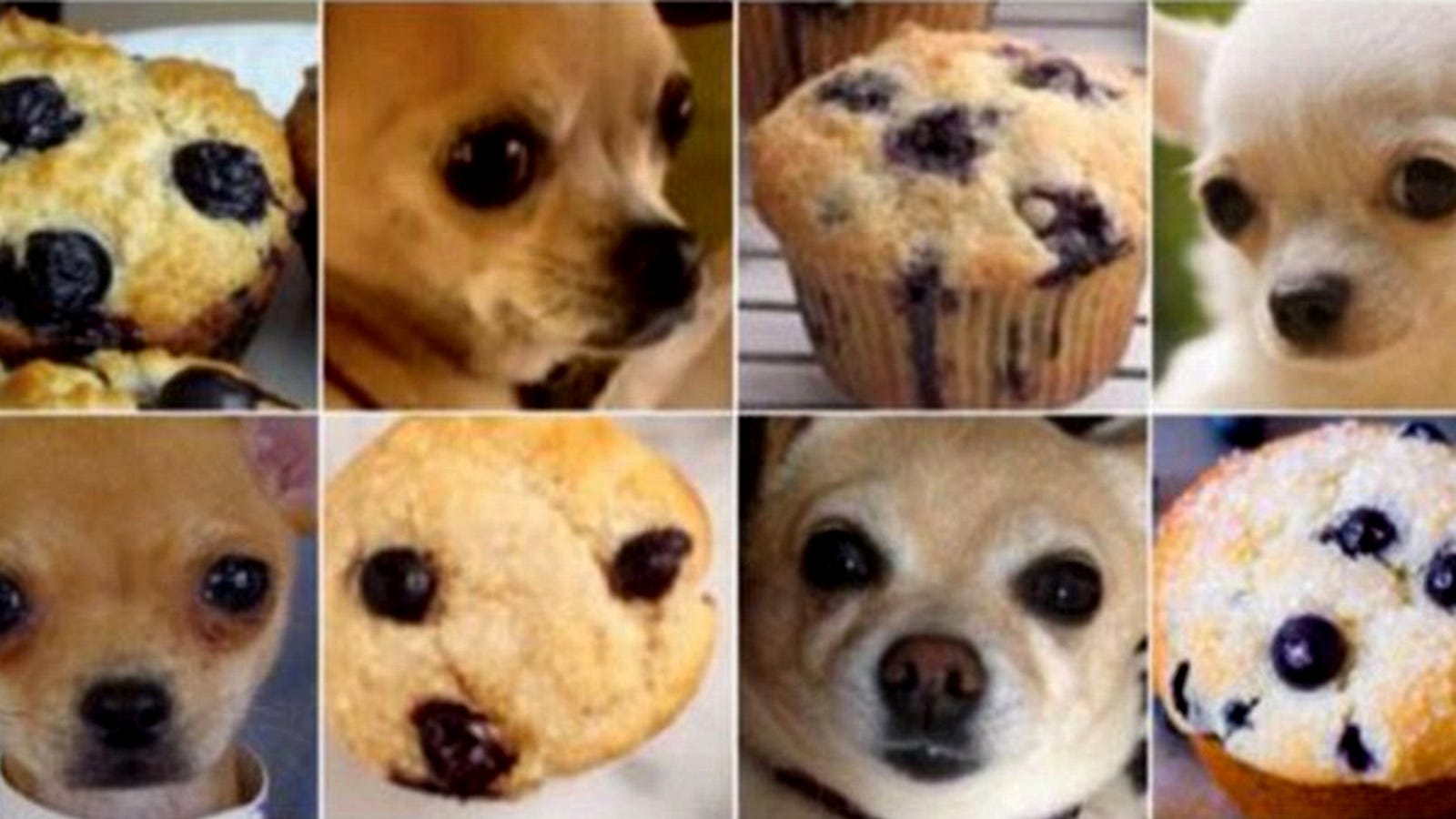
Neural networks form the core of deep learning, a subset of machine learning that I introduced in my previous article. People exposed to artificial intelligence generally have a good high-level idea of how a neural network works — data is passed from one layer of the neural network to the next, and this data is propagated from the topmost layer to the bottom layer until, somehow, the algorithm outputs the prediction on whether an image is that of a chihuahua or a muffin.
Seems like magic, isn’t it? Surprisingly, neural networks for a computer vision model can be understood using high school math. It just requires the correct explanation in the simplest manner for everyone to understand how neural networks work under the hood. In this article, I will utilise the MNIST handwritten digit database to explain the process of creating a model utilising neural networks from the ground up.
Before we dive in, it’s important to highlight just why we need to understand how neural networks work under the hood. Any aspiring machine learning developer could simply utilise 10 lines of code 👇 to differentiate between cats and dogs — so why bother learning what goes on underneath?
Here’s my take: without a complete grasp of what are neural networks in machine learning, we will 1) never be able to customise the code needed fully, and adapt it for different problems in the real world, and 2) debugging will be a nightmare.
Simply put, a beginner using a complex tool without understanding how the tool works is still a beginner until he fully understands how most things work.
In this article, We’ll cover the following:
Neural Network: Computer-Generated Prediction
To completely understand this, we have to go back to where the term “Machine Learning” was first popularised.
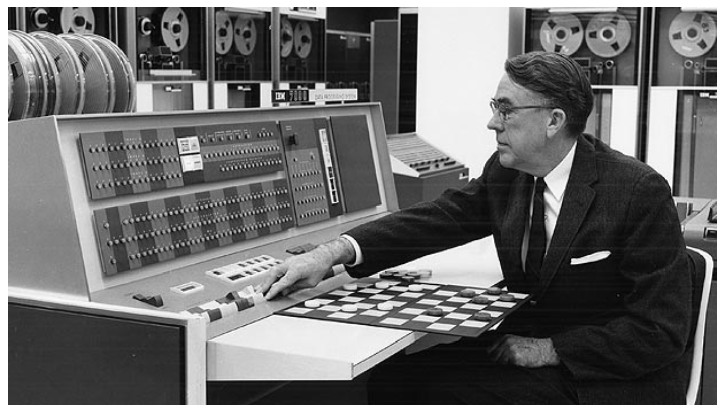
According to Arthur Samuel, one of the early pioneers in artificial intelligence, and creator of one of the world’s first successful self-learning programs, he defined machine learning as:
Suppose we arrange for some automatic means of testing the effectiveness of any current weight assignment in terms of actual performance and provide a mechanism for altering the weight assignment so as to maximize the performance. We need not go into the details of such a procedure to see that it could be made entirely automatic and to see that a machine so programmed would “learn” from its experience.
From this quote, we can identify 7 fundamental steps in machine learning. Taken within the context of identifying between any two handwritten digits “2” or “9”:
- Initialise the weights
- For each image, use these weights to predict whether it is a 2 or a 9.
- Out of all these predictions, find out how good the model is.
- Calculating the gradient, which measures for each weight, how changing the weight would change the loss
- Change all weights based on the calculation
- Go back to step 2 and repeat
- Iterate until the decision to stop.
We can visualize the flow of these 7 steps in the following diagram:
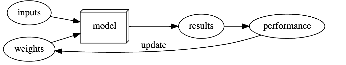
Yes, looking at this can be slightly overwhelming, since there are tons of new technical jargon that might be unfamiliar. What are weights? What are epochs? Just stick with me, I’ll explain these in a step-by-step fashion down below. These steps might not make a lot of sense, but just hang tight!
The Prerequisites — Importing, Processing the Data
First, let us do all the prerequisites — importing the necessary packages. This is the most basic step in beginning to create any computer vision model. We will be using PyTorch as well as fast.ai. Since fast.ai is a library that is built on top of PyTorch, this article will explain how some of the fast.ai built-in functions are written (for example, the learner class in line 9 of the above list).
from fastai.vision.all import *
from fastbook import *
Second, let’s grab the images from the MNIST dataset. For this particular example, we have to retrieve the data from the training directories of handwritten numbers 2 and 9.
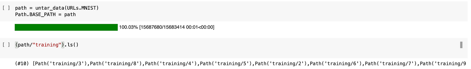
To find out what the folder contains, we can employ the use of the .ls() function in fast.ai. Then, we open the images to check out what it looks like-
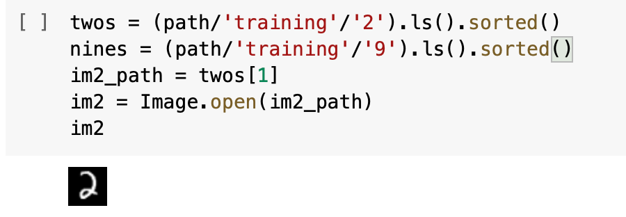
As you can see, it’s simply an image of the handwritten number ‘2’!
However, computers are unable to recognise images that are passed into them just like that — data in the computer is represented as a set of numbers. We can illustrate that in the example here:
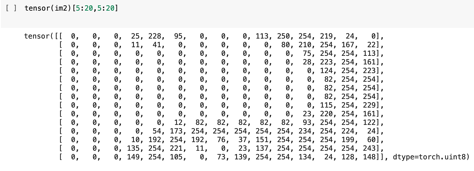
Now, what do all these numbers represent? Let’s take a look at it using a handy function that pandas provide us with:
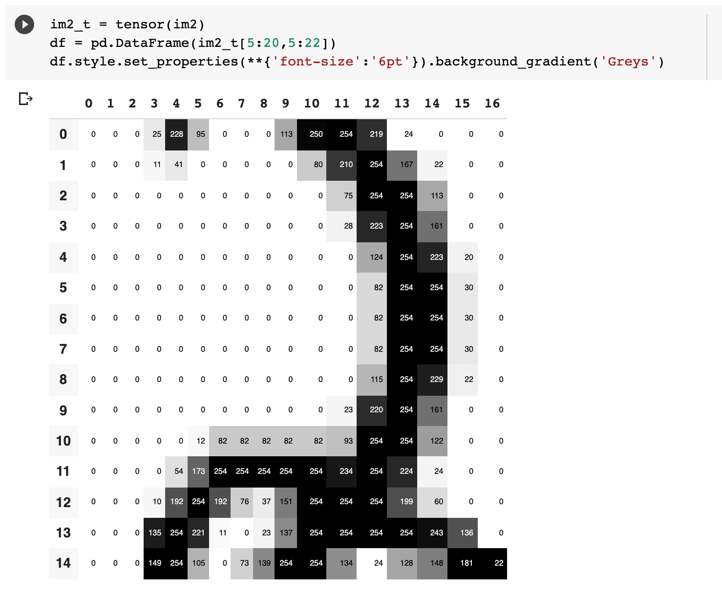
As shown above, the main way that computers interpret images is through the form of pixels, which are the smallest building blocks of any computer display. These pixels are recorded in the form of numbers.
Now that we have a better understanding of how the computer truly interprets the images, let’s dive into how we can manipulate the data to give our prediction.
Data Structures and Data Sets
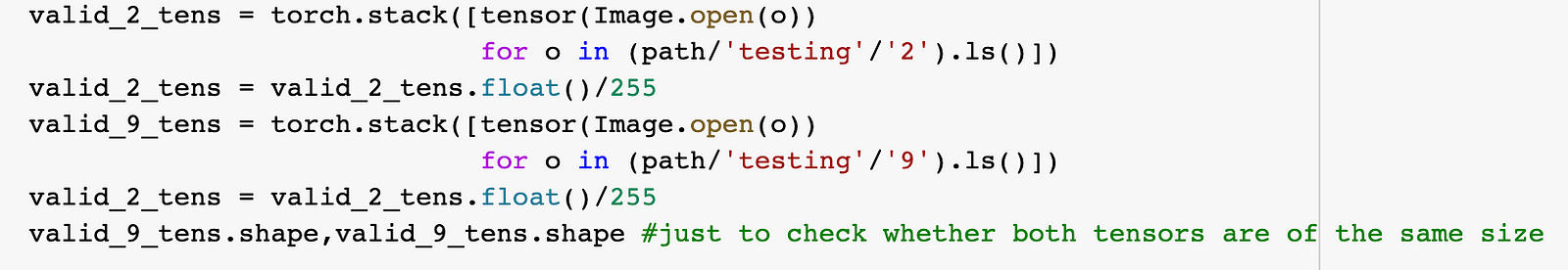
Before even calculating the predictions we have to ensure that the data is structured in the same way for the program to process all the different images. Let’s make sure that we have two different tensors, each for all of the ‘nines’ and ‘twos’ in the dataset.
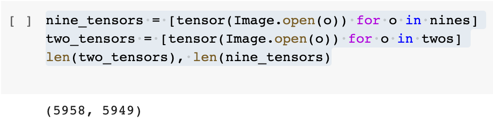

Before progressing further, we have to discuss what exactly is a tensor. I first heard of the word tensor in the name TensorFlow, which is a (completely!) separate library from which we are using. A PyTorch Tensor in this case is a multidimensional table of data, with all data items of the same type. The difference between lists or arrays and PyTorch Tensors is that these tensors can finish computations much (many thousands of times) faster than using conventional Python arrays.
Parsing all the data that we have collected as training data to the model isn’t going to cut it — simply because we need something to check our model against. We don’t want our model to overtrain or overfit our training data, performing well in training, only to break when it encounters something that it has never seen before, outside of the training data. Therefore, we have to split the data into the training dataset and the validation dataset.
To do this, we do:
In addition, we have to create variables — both independent variables and dependent variables to allow such data to be tracked.
train_x = torch.cat([stacked_twos, stacked_nines]).view(-1, 28*28)
This train_x variable will hold all of our images as independent variables (i.e., what we want to measure, think: 5th-grade science!).
We then create the dependent variable, assigning the value ‘1’ to represent the handwritten twos, with the value ‘0’ to represent the handwritten nines in the data.
train_y = tensor([1]*len(twos) + [0]*len(nines)).unsqueeze(1)
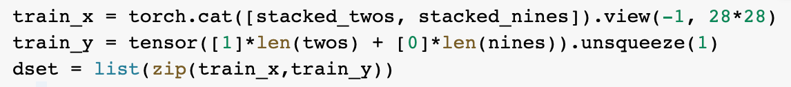
We then create a dataset based on the independent and dependent variables, combining them into a tuple, a form of immutable lists.
We then repeat the process for the validation dataset:
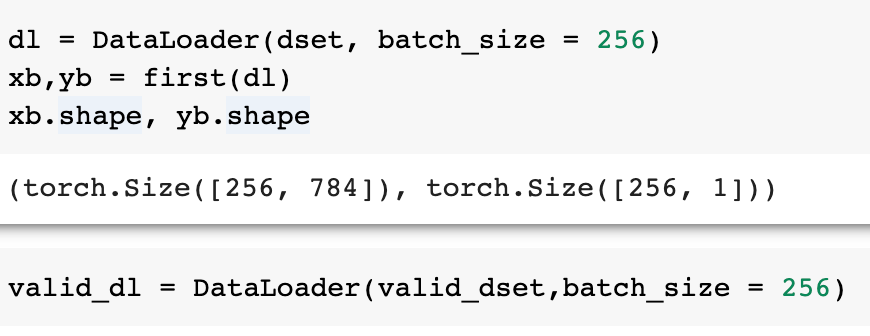
We then go about loading both datasets into a DataLoader with the same batch size.
Now that we have completed the set-up of our data, we can go about processing this data with our model.
Creating a Layer Linear Model
We have completed the setup of our data. Circling back to the seven steps of machine learning, we can slowly work our way through them now.
Step 1: Initialising the weights
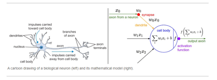
What are weights? Weights are variables, and a weight assignment is a particular choice of values for those variables. It can be thought of the emphasis that is given to each data point for the program to work. In other words, changing these sets of weights will change the model to behave differently for a different task.
Here, we initialise the weights randomly for every pixel —
Pls, check if something is missing from here -?
Together, the weights and biases (present because weights could sometimes be zero, and we want to prevent that) make up the parameters.
There was something that bothered me — was there a better way to initialise the weights, as compared to dumping a random number in?
It turns out that random initialisation in neural networks is a specific feature, not a mistake. In this case, stochastic optimisation algorithms (which will be explained below) use randomness in selecting a starting point in the search before progressing down the search.
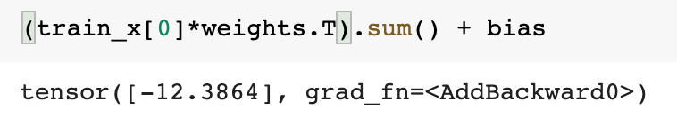
Step 2: Predictions — for each image, predict whether this is a 2 or a 9.
We can then go ahead and calculate our first-ever prediction:
Following that, we calculate the predictions for the rest of the data using mini-batches:
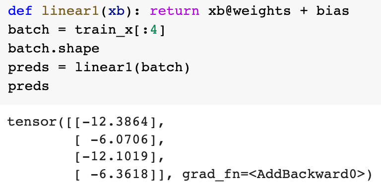
👆This step is crucial, due to it having the ability to calculate the predictions, and is one of the two fundamental equations of any neural network.
Step 3: Utilising the loss function to understand how good our model is
To find out how good the model is, we have to use a loss function. This is the clause “testing the effectiveness of any current weight assignment in terms of actual performance”, and is the premise on how the model will update its weights to give a better prediction.
Think about a basic loss function. We can’t use accuracy as a loss function because the accuracy will only change if the predictions of whether an image is either a ‘2’ or a ‘9’ change completely — in that sense, accuracy wouldn’t catch the small updates on the confidence or certainty with which the model is predicting the results.
What we can do, however, is to create a function that records the difference between the predictions that the model gives (for example — it gives 0.2 for a fairly certain prediction that the image that it is interpreting is closer to 2 rather than 9) and the actual label associated with it (in this case, it would be 0, therefore the raw difference, the loss, between the prediction and the model would be 0.2).
BUT wait! As you can see from the output, not all predictions will lie in the range between 0 and 1, some of them might be far off. What we want is another function that can squish the values between 0 and 1.
Well, there’s a handy function for this — it’s called the Sigmoid Function. It is a mathematical function that is given by (1/ 1+e^(-x)) that contains all numbers, positive and negative between 0 and 1.
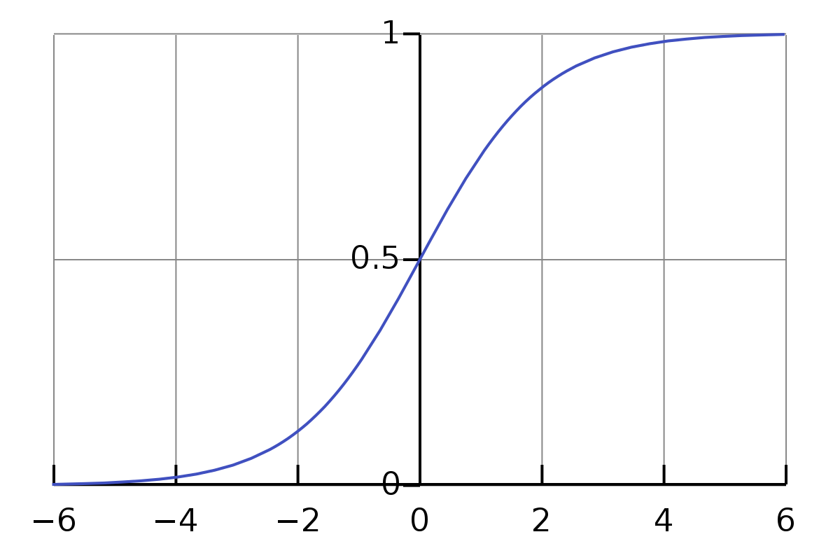
Now, there may be a misconception that some people have when learning Machine Learning through introductory videos — I certainly had some. If you google online, the Sigmoid function is generally frowned upon, but it is important to know the context in which the Sigmoid function is used before criticising it. In this case, it is used merely as a way to compress the numbers between 0 and 1 for the loss function. We are not using Sigmoid as an activation function, which would be discussed later.
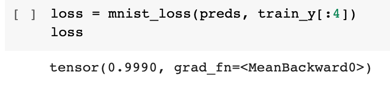
We can therefore calculate the loss for our mini-batch:
Step 4: Calculating the gradient — The Principle of Stochastic Gradient Descent
Since we might start with any given weights (random weights), the point of the machine learning model is to reach the lowest possible loss within the training limits of the model.
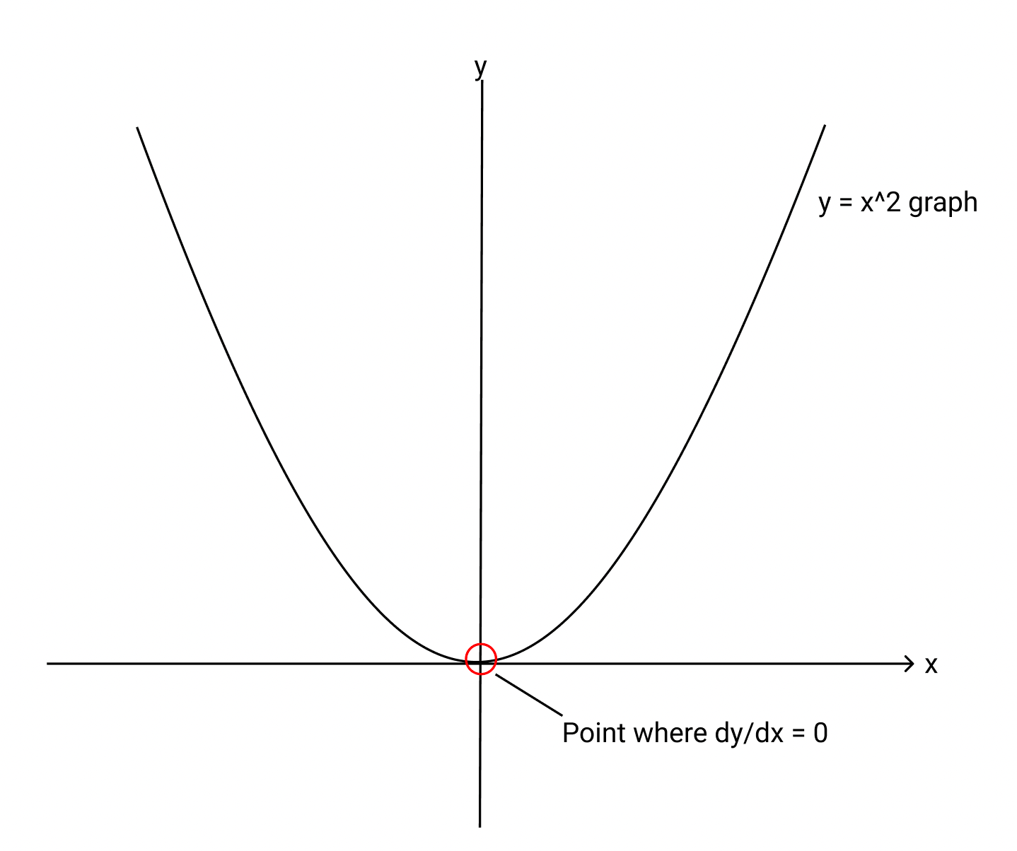
This might sound complex, but it only requires high school math to have a good understanding of this concept. Imagine we have our loss function is an arbitrary quadratic function y = x², and we want to minimise this loss function. We would immediately think of the point where the derivative or the gradient of this function is zero, which happens to be at the lowest point (or the “valley”). Drawing a line tangential to the curve at that point would give us a straight line. We would want the program to constantly update itself to reach that minimum point.
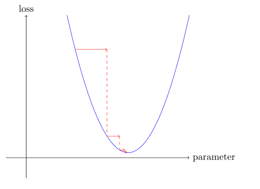
This is one of the primary ways that loss is minimized in machine learning, and it provides a broad overview of how the training of models is sped up rapidly.
To calculate the gradients (no, we don’t have to do it manually, so you wouldn’t need to dig up your high school math notes), we write the following function:
Step 5: Changing the weights based off the calculated gradient (stepping the weights)
If you’ve made it this far, that’s it! These are the raw steps written that are needed to train the model once, in a linear fashion. Steps 1 through 5 are the fundamental steps that are needed to go through the data once, and the period of running through the data once is called “epoch”.
The difference between stochastic gradient descent (SGD) and gradient descent (GD) is the line “for xb,yb in dl” — SGD has it, while GD does not. Gradient descent will calculate the gradient of the whole dataset, whereas SGD calculates the gradient on mini-batches of various sizes.
Now, for simplicity’s sake, we consolidate all the other functions (validation, accuracy) that we have written into higher-level functions, and put the various batches together:
Step 6: Repeating from Step 2

Yay! We have just built a linear (one-layer) network that can train, within a really short time, to a crazy level of accuracy.
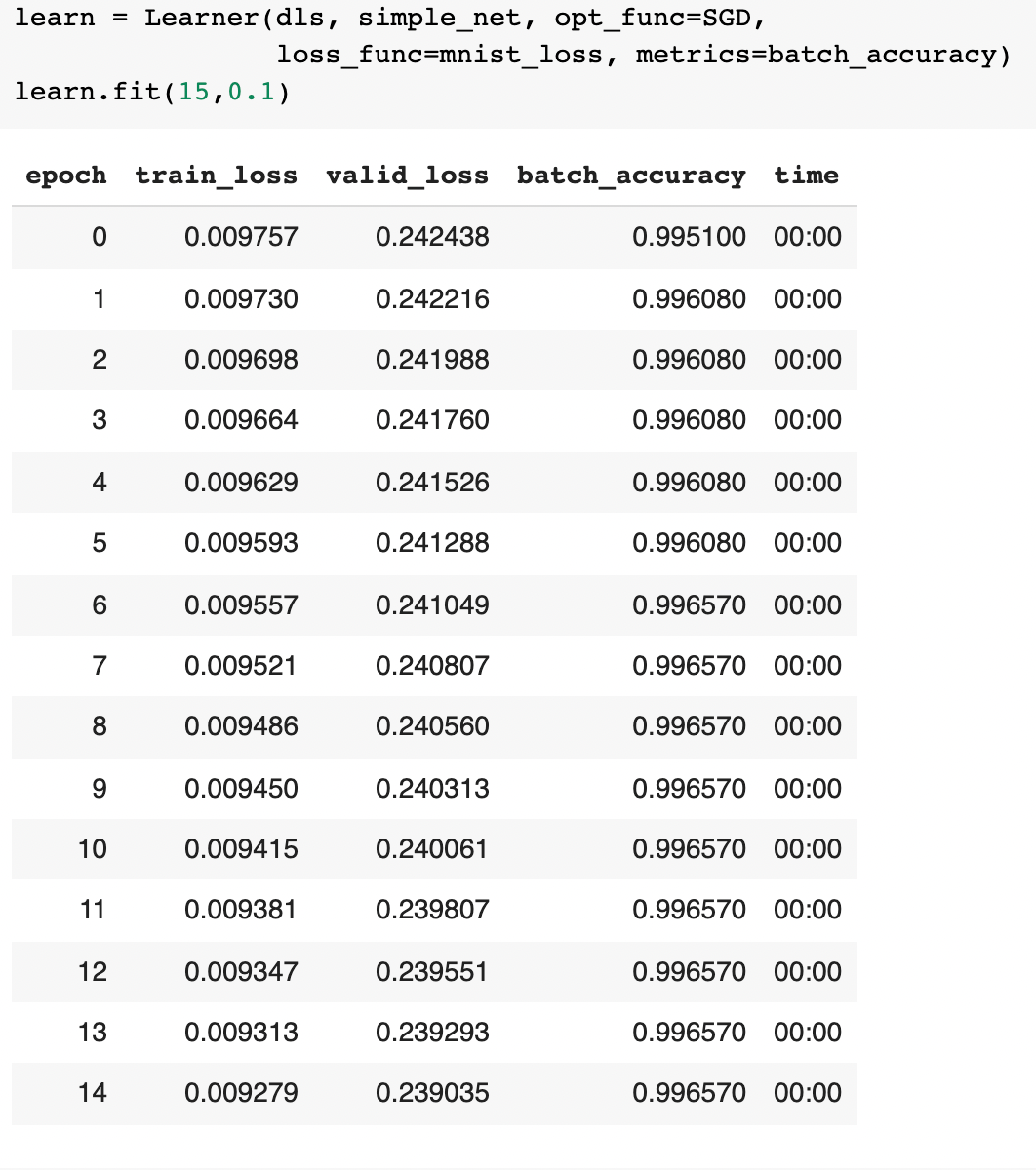
To optimise this process and reduce the amount of lower-level functions (and to make our code look a little nicer, of course) — we use the pre-built in functions (e.g. a class called Learner) which have the same functionality as the lines of code before.
Creating multiple layers using the activation function
How do we progress from a linear layered program to one of the multiple layers? The key lies in a simple line of code –
This is known as an activation function, one which combines two linear layers to make it into a two-layered network.
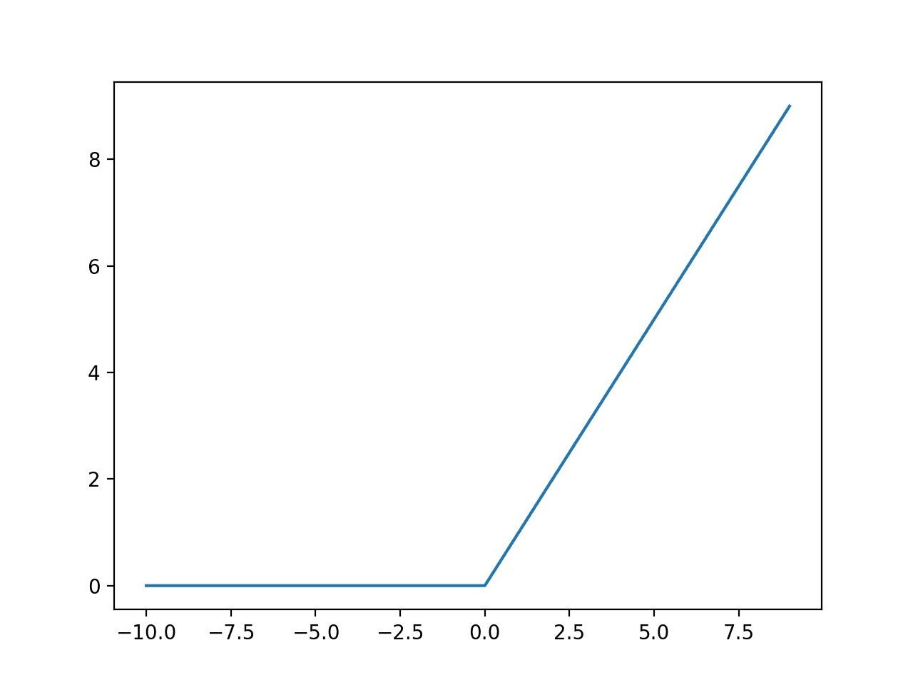
In particular, this res.max function is also known as a rectified linear unit (ReLU), which is a fancy way of saying “convert all negative numbers to zero and leave the positive numbers as they are”. This is one such activation function, while there are many others out there — such as Leaky ReLU, Sigmoid (frowned upon to be used specifically as an activation function), tanh, etc.
Now that we understand how to combine two different linear layers, we can now create a simple neural network out of it:
And then we can finally train our model using our two-layered artificial neural network:
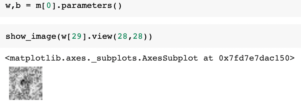
What’s even more interesting is that we can even see what images the model is trying to process in the various layers of this simple net architecture!
Conclusion
Understanding what goes inside an artificial neural network might seem daunting at first. Neural networks are the key to customization and understanding which parts of the model went wrong if we do have to build a model right from scratch. What it takes is simply determination, a working computer, and some very rudimentary understanding of high school math concepts to dive deep into AI.
If you want to play around with the code and see how it all works, hit this link to try it out yourself! Alternatively, you could check out my Github repository here: https://github.com/danielcwq/mnist2-9/blob/main/mnist2_9.ipynb
If you want to know more about neural networks. Feel free to reach out to me at my website!
The media shown in this article is not owned by Analytics Vidhya and are used at the Author’s discretion.


Thank you so much for sharing! Trying to dive into this field for healthcare applications but still a begginer. Surelly understandign what is happening behind the code helps a Lot.
In the middle of the article there is a text bit looking like an editor's note "pls check if something is missing here".