Introduction:
We live in a fast changing digital world. In today’s age customers expect the sellers to tell what they might want to buy. I personally end up using Amazon’s recommendations almost in all my visits to their site.
This creates an interesting threat / opportunity situation for the retailers.
If you can tell the customers what they might want to buy – it not only improves your sales, but also the customer experience and ultimately life time value.
On the other hand, if you are unable to predict the next purchase, the customer might not come back to your store.
In this article, we will learn one such algorithm which enables us to predict the items bought together frequently. Once we know this, we can use it to our advantage in multiple ways.
Table of contents
1. The Approach(Apriori Algorithm)
When you go to a store, would you not want the aisles to be ordered in such a manner that reduces your efforts to buy things?
For example, I would want the toothbrush, the paste, the mouthwash & other dental products on a single aisle – because when I buy, I tend to buy them together. This is done by a way in which we find associations between items.
In order to understand the concept better, let’s take a simple dataset (let’s name it as Coffee dataset) consisting of a few hypothetical transactions. We will try to understand this in simple English.
The Coffee dataset consisting of items purchased from a retail store.
Coffee dataset:

The Association Rules:
For this dataset, we can write the following association rules: (Rules are just for illustrations and understanding of the concept. They might not represent the actuals).
Rule 1: If Milk is purchased, then Sugar is also purchased.
Rule 2: If Sugar is purchased, then Milk is also purchased.
Rule 3: If Milk and Sugar are purchased, Then Coffee powder is also purchased in 60% of the transactions.
Generally, association rules are written in “IF-THEN” format. We can also use the term “Antecedent” for IF (LHS) and “Consequent” for THEN (RHS).
From the above rules, we understand the following explicitly:
- Whenever Milk is purchased, Sugar is also purchased or vice versa.
- If Milk and Sugar are purchased then the coffee powder is also purchased. This is true in 3 out of the 5 transactions.
For example, if we see {Milk} as a set with one item and {Coffee} as another set with one item, we will use these to find sets with two items in the dataset such as {Milk,Coffee} and then later see which products are purchased with both of these in our basket.
Therefore now we will search for a suitable right hand side or Consequent. If someone buys Coffee with Milk, we will represent it as {Coffee} => {Milk} where Coffee becomes the LHS and Milk the RHS.
When we use these to explore more k-item sets, we might find that {Coffee,Milk} => {Tea}.
That means the people who buy Coffee and Milk have a possibility of buying Tea as well.
Let us see how the item sets are actually built using the Apriori.
| LHS | RHS | Count |
| Milk | – | 300 |
| Coffee | – | 200 |
| Tea | – | 200 |
| Sugar | – | 150 |
| Milk | Coffee | 100 |
| Tea | Sugar | 80 |
| Milk, Coffee | Tea | 40 |
| Milk, Coffee, Tea | Sugar | 10 |
Apriori envisions an iterative approach where it uses k-Item sets to search for (k+1)-Item sets. The first 1-Item sets are found by gathering the count of each item in the set. Then the 1-Item sets are used to find 2-Item sets and so on until no more k-Item sets can be explored; when all our items land up in one final observation as visible in our last row of the table above. One exploration takes one scan of the complete dataset.
An Item set is a mathematical set of products in the basket.
1.1 Handling and Readying The Dataset
The first part of any analysis is to bring in the dataset. We will be using an inbuilt dataset “Groceries” from the ‘arules’ package to simplify our analysis.
All stores and retailers store their information of transactions in a specific type of dataset called the “Transaction” type dataset.
The ‘pacman’ package is an assistor to help load and install the packages. we will be using pacman to load the arules package.
The p_load() function from “pacman” takes names of packages as arguments.
If your system has those packages, it will load them and if not, it will install and load them.
Example:
pacman::p_load(PACKAGE_NAME)pacman::p_load(arules, arulesViz)OR
Library(arules)Library(arulesViz)data(“Groceries")1.2 Structural Overview and Prerequisites
Before we begin applying the “Apriori” algorithm on our dataset, we need to make sure that it is of the type “Transactions”.
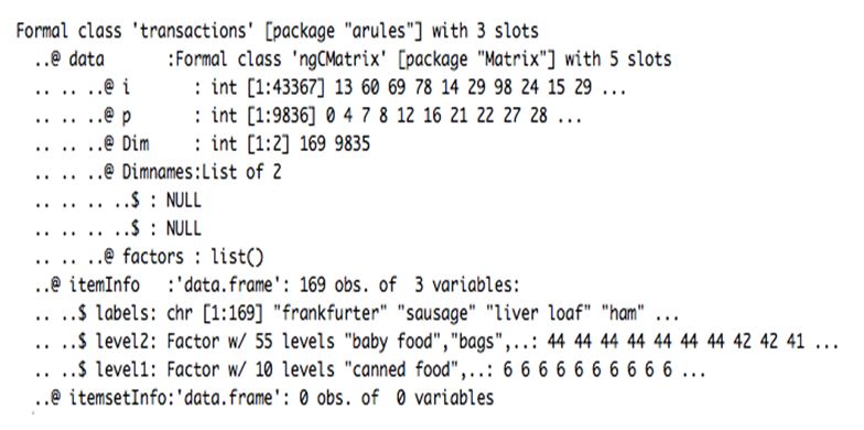
str(Groceries)The structure of our transaction type dataset shows us that it is internally divided into three slots: Data, itemInfo and itemsetInfo.
The slot “Data” contains the dimensions, dimension names and other numerical values of number of products sold by every transaction made.

These are the first 12 rows of the itemInfo list within the Groceries dataset. It gives specific names to our items under the column “labels”. The “level2” column segregates into an easier to understand term, while “level1” makes the complete generalisation of Meat.
The slot itemInfo contains a Data Frame that has three vectors which categorizes the food items in the first vector “Labels”.
The second & third vectors divide the food broadly into levels like “baby food”,”bags” etc.
The third slot itemsetInfo will be generated by us and will store all associations.

This is what the internal visual of any transaction dataset looks like and there is a dataframe containing products bought in each transaction in our first inspection. Then, we can group those products by TransactionID like we did in our second inspection to see how many times each is sold before we begin with associativity analysis.
The above datasets are just for a clearer visualisation on how to make a Transaction Dataset and can be reproduced using the following code:
data <- list(
c("a","b","c"),
c("a","b"),
c("a","b","d"),
c("b","e"),
c("b","c","e"),
c("a","d","e"),
c("a","c"),
c("a","b","d"),
c("c","e"),
c("a","b","d","e"),
c("a",'b','e','c')
)
data <- as(data, "transactions")
inspect(data)
#Convert transactions to transaction ID lists
tl <- as(data, "tidLists")
inspect(tl)
Let us check the most frequently purchased products using the summary function.
summary(Groceries)

The summary statistics show us the top 5 items sold in our transaction set as “Whole Milk”,”Other Vegetables”,”Rolls/Buns”,”Soda” and “Yogurt”. (Further explained in Section 3)
To parse to Transaction type, make sure your dataset has similar slots and then use the as() function in R.
2. Implementing Apriori Algorithm and Key Terms and Usage
rules <- apriori(Groceries,parameter = list(supp = 0.001, conf = 0.80))We will set minimum support parameter (minSup) to .001.
We can set minimum confidence (minConf) to anywhere between 0.75 and 0.85 for varied results.
I have used support and confidence in my parameter list. Let me try to explain it:
Support: Support is the basic probability of an event to occur. If we have an event to buy product A, Support(A) is the number of transactions which includes A divided by total number of transactions.
Confidence: The confidence of an event is the conditional probability of the occurrence; the chances of A happening given B has already happened.
Lift: This is the ratio of confidence to expected confidence.The probability of all of the items in a rule occurring together (otherwise known as the support) divided by the product of the probabilities of the items on the left and right side occurring as if there was no association between them.
The lift value tells us how much better a rule is at predicting something than randomly guessing. The higher the lift, the stronger the association.
Let’s find out the top 10 rules arranged by lift.
inspect(rules[1:10])

As we can see, these are the top 10 rules derived from our Groceries dataset by running the above code.
The first rule shows that if we buy Liquor and Red Wine, we are very likely to buy bottled beer. We can rank the rules based on top 10 from either lift, support or confidence.
Let’s plot all our rules in certain visualisations first to see what goes with what item in our shop.
3. Interpretations and Analysis
Let us first identify which products were sold how frequently in our dataset.
3.1 The Item Frequency Histogram
These histograms depict how many times an item has occurred in our dataset as compared to the others.
The relative frequency plot accounts for the fact that “Whole Milk” and “Other Vegetables” constitute around half of the transaction dataset; half the sales of the store are of these items.

arules::itemFrequencyPlot(Groceries,topN=20,col=brewer.pal(8,'Pastel2'),main='Relative Item Frequency Plot',type="relative",ylab="Item Frequency (Relative)")This would mean that a lot of people are buying milk and vegetables!
What other objects can we place around the more frequently purchased objects to enhance those sales too?
For example, to boost sales of eggs I can place it beside my milk and vegetables.
3.2 Graphical Representation
Moving forward in the visualisation, we can use a graph to highlight the support and lifts of various items in our repository but mostly to see which product is associated with which one in the sales environment.
plot(rules[1:20],method = "graph",control = list(type = "items"))This representation gives us a graph model of items in our dataset.
The size of graph nodes is based on support levels and the colour on lift ratios. The incoming lines show the Antecedants or the LHS and the RHS is represented by names of items.

The above graph shows us that most of our transactions were consolidated around “Whole Milk”.
We also see that all liquor and wine are very strongly associated so we must place these together.
Another association we see from this graph is that the people who buy tropical fruits and herbs also buy rolls and buns. We should place these in an aisle together.
3.3 Individual Rule Representation
The next plot offers us a parallel coordinate system of visualisation. It would help us clearly see that which products along with which ones, result in what kinds of sales.
As mentioned above, the RHS is the Consequent or the item we propose the customer will buy; the positions are in the LHS where 2 is the most recent addition to our basket and 1 is the item we previously had.

The topmost rule shows us that when I have whole milk and soups in my shopping cart, I am highly likely to buy other vegetables to go along with those as well.
plot(rules[1:20],method = "paracoord",control = list(reorder = TRUE))If we want a matrix representation, an alternate code option would be:
plot(rules[1:20],method = "matrix",control = list(reorder = TRUE)3.4 Interactive Scatterplot
These plots show us each and every rule visualised into a form of a scatterplot. The confidence levels are plotted on the Y axis and Support levels on the X axis for each rule. We can hover over them in our interactive plot to see the rule.

Plot: arulesViz::plotly_arules(rules)
The plot uses the arulesViz package and plotly to generate an interactive plot. We can hover over each rule and see the Support, Confidence and Lift.
As the interactive plot suggests, one rule that has a confidence of 1 is the one above. It has an exceptionally high lift as well, at 5.17.
How does the Apriori algorithm work?
- Step 1 – Find frequent items:
- It starts by identifying individual items (like products in a store) that appear frequently in the dataset.
- Step 2 – Generate candidate itemsets:
- Then, it combines these frequent items to create sets of two or more items. These sets are called “itemsets”.
- Step 3 – Count support for candidate itemsets:
- Next, it counts how often each of these itemsets appears in the dataset.
- Step 4 – Eliminate infrequent itemsets:
- It removes itemsets that don’t meet a certain threshold of frequency, known as the “support threshold”. This threshold is set by the user.
- Repeat Steps 2-4:
- The process is repeated, creating larger and larger itemsets, until no more can be made.
- Find associations:
- Finally, Apriori uses the frequent itemsets to find associations. For example, if “bread” and “milk” are often bought together, it will identify this as an association.
FAQs
Q1. How can we make the Apriori algorithm more efficient?
1. Use hash tables and transaction reduction to reduce scanning.
2. Partition the dataset and sample a subset to improve scalability.
3. Use dynamic counting, early termination, and parallelization to optimize computations.
4. Employ data compression and specialized hardware for further efficiency gains.
Q2. Which is better Apriori or FP growth?
FP-Growth is generally considered more efficient than Apriori for large datasets due to its ability to mine frequent itemsets with fewer scans of the data. Apriori may be a better choice for smaller datasets or when simplicity is a priority.
Q3. What are the factors affecting Apriori algorithm?
1.Larger datasets increase complexity and execution time.
2. More items increase candidate itemsets to evaluate.
3. Higher support reduces frequent itemsets but increases candidate itemsets.
4. Wider transactions increase itemsets and impact performance.
5.Sparser data makes it harder to identify frequent itemsets.
End Notes and Summary
By visualising these rules and plots, we can come up with a more detailed explanation of how to make business decisions in retail environments.
Now, we would place “Whole Milk” and “Vegetables” beside each other; “Wine” and “Bottled Beer” alongside too.
I can make some specific aisles now in my store to help customers pick products easily from one place and also boost the store sales simultaneously.
Aisles Proposed:
- Groceries Aisle – Milk, Eggs and Vegetables
- Liquor Aisle – Liquor, Red/Blush Wine, Bottled Beer, Soda
- Eateries Aisle – Herbs, Tropical Fruits, Rolls/Buns, Fruit Juices, Jams
- Breakfast Aisle – Cereals, Yogurt, Rice, Curd
This analysis would help us improve our store sales and make calculated business decisions for people both in a hurry and the ones leisurely shopping.
Happy Association Mining!


HI Shantanu Kumar, Thanks for the great post on Apriori. I want to know how does it work with big data set of transactions (eg. more than 4 GB in size of file.)
The Algorithm will first create all associativity rules from any Transactional Type Dataset, then statically access those using Breadth First Search. I believe 4GB will not create any issues in processing, as once the rules are created you only have to access them in O(1) if you know your LHS. If you want, you can send across the dataset and I'll look into it.
Good Day Shantanu Kumar: Thanks for your posting. I learned new possibilities to Association Rules. I have a technical question. I noticed that for some odd reason if I use the read,transactions function with a csv file the results will differ if I use it against a transaction set extracted from a Database table( using the package RODBC) in both cases is reading using the same structure. I do not know if you had that experience and could give some lights about it. Thanks in advance
Hi! Thanks a lot for the appreciation, glad it was of some use to you :) I've had a similar problem and there's usually the issue because of the functions that you use. The packages have described each function in their own way, so the internal processing for different package functions may be different. Try looking at the source code for those functions or show me your output datasets and I'll help you solve the issue.
Are you familiar with steps that remove redundant rules? I've seen several different approaches to them but each kind of do a different thing and nobody can seem to answer this.
Hi, there's two ways to approach redundancy. One is through the raw code where you scan each item and check for redundancies. The other and easier method is to use the "is.redundant()" function on your rules to identify them one by one for the same. Hope this answers your doubt.