Invert the characteristics of Convolution with Involution

Introduction

Convolution operation reigned supreme in the domain of computer vision. Deep Convolutional Neural Network Architectures are the de facto models for solving vision-related tasks. They achieved SOTA performance in several benchmarks and dominated the Vision Domain for the past few years. Self Attention Based models following their massive success in Natural Language Processing domain are finding increasingly many applications in vision-related tasks. In these really exciting times another great neural network primitive operation was proposed by Duo Li, Jie Hu, Changhua Wang, Xiangtai Li, Qi She, Lei Zhu, Tong Zhang, Qifeng Chen(researchers at The Hong Kong University of Science and Technology, ByteDance AI Lab and Peking University) on 11 April 2021. In this post let’s explore the involution.

Dissecting the Convolution

Convolution (also called composition product, superposition integral, Carson’s integral) is the most important operation in Signal processing. It is a way to combine two signals to get the third signal. As Images are nothing but two-dimensional signals convolution finds applications in vision-related tasks. Mathematically Convolution is given by:

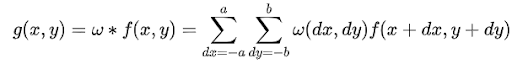
Here f is our input image and w is some other 2D matrix(of size (2a,2b)) called kernel or filter or mask. Before exploring the contents of w and its effects on input image via convolution, let’s see how to calculate convolution given matrices(“ * ” is the convolution operator).

Pseudo Code:

for each pixel in image row:
set accumulator to zero
for each kernel row in kernel:
for each element in kernel row:
if element position corresponding* to pixel position then
multiply element value corresponding* to pixel value
add result to accumulator
endif
set output image pixel to accumulator

The kernel is usually smaller than the image and it is slid across the image to generate each output pixel value. We can control the output shape by controlling how fast the kernel slides(stride) and the padding around the input image.

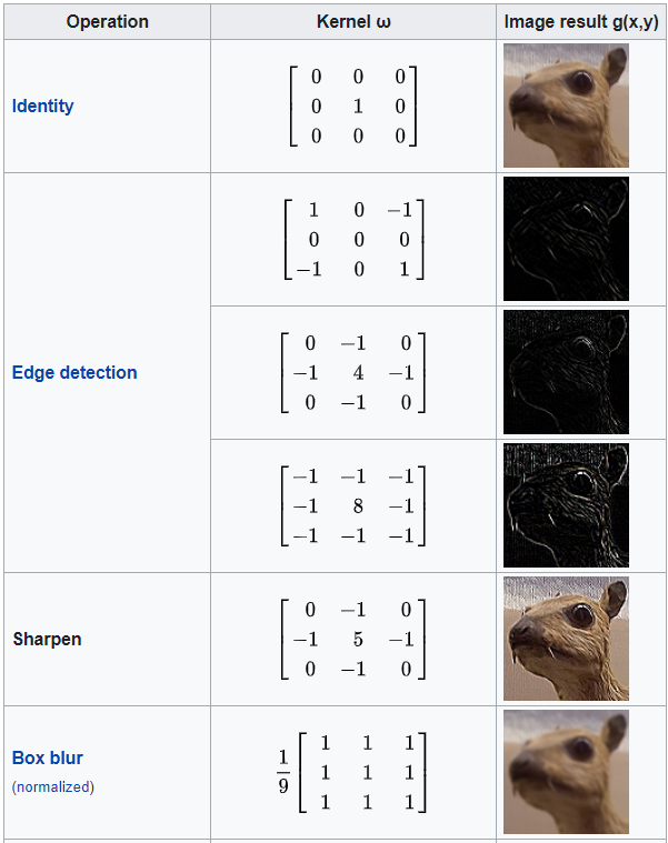
What is this w Matrix? It can be anything depending on what we want the output of the convolution to be. To get a better understanding let’s see some example kernels and their effects on images.

Convolution gained popularity as a neural network primitive owing to its Shape agnostic and channel-specific behavior. Let’s demystify these behaviors.

Translational Equivalence

Convolution describes the output of a Linear Time-Invariant(LTI) class of operations. Time invariance translates to spatial invariance when we talk about 2D images. This in turn lets us model systems with translational equivalence as convolutions.

For Example, when we need to identify a shape in an image, we need the system to be shift-invariant i.e. wherever the shape is in the image it would be detected. Convolution is a natural choice for modelling such systems as we slide the same kernel over the image.

Channel Specific Behavior

Different channels of images contain diverse information encoded in them. Therefore using a different convolution kernel for every image channel allows us to extract this diverse information.

This line of reasoning was believed to be accurate for several years. But in the latest model architectures, it is found that there is inter-channel redundancy amongst channels-specific convolutional kernels. This casts a doubt on the widely successful channel-specific convolutional kernels.

Typical Convolutional Neural network Architecture

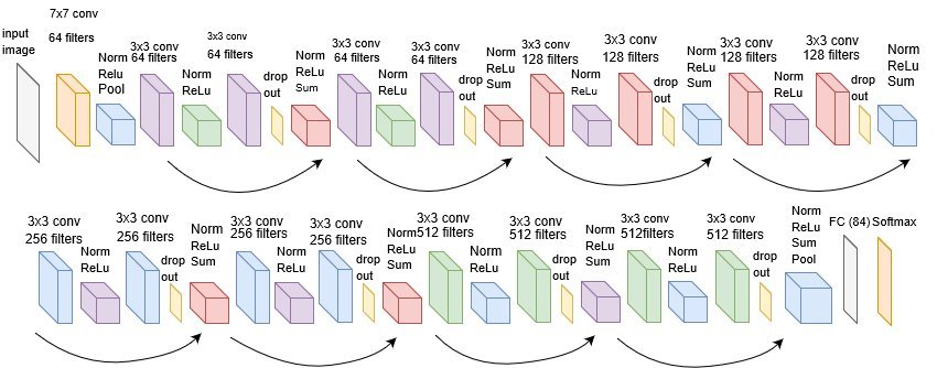
Cohort Kernels are used to extract feature maps in each layer of the Neural Network. The number of feature maps extracted are equal to the number of kernels or filters. Output shape is dependent on stride and padding. Each of these feature maps is considered to be a channel of the input for the next step.

The linear nature of convolution makes stacking them useless as stacked linear layers necessarily are equivalent to a single layer. This can be handled simply by adding a nonlinear activation like RELU. Shown above is the architecture of ResNet 18 which is one of the most successful lightweight Neural Networks for vision tasks.

Disadvantages of Convolution

The biggest disadvantage of Convolution is the inherent locality constraints. Convolution is limited in its ability to extract visual patterns across different spatial positions. The receptive field of each pixel is narrow making it very hard to model long-range multihop dependencies amongst the pixels.

Self Attention

Attention is another revolutionary NN primitive that transformed Natural Language Processing as a part of the Transformer Architecture. Its variations are being adopted in disparate domains at an unprecedented rate. However, its quadratic computational complexity limits its usage in Image related tasks. The main idea of self-attention is to do non-local filtering of the image with weights based on the similarity of the pixels.

The Q,K,V vectors are generated for each pixel using few Linear layers. This is game-changing as each out pixel is calculated by considering all the input pixels. The complexity is O(N4) for N*N input. This fills up the memory quite fast and also takes a lot of time to compute. Although novel approaches like using low dimensional learned latent arrays(Perceiver), Axial attention(Medical Transformer), etc. bring this wonderful operation into Vision Architectures there is still a lot of scopes to improve. We will see that involution is a more general representation of Attention.

Involution

The idea of Involution is to invert the characteristics of Convolution. Involution computation is the same as convolution except for the kernel. Unlike in Convolution, a single learned kernel is not slid over the image. The kernel is dynamically instantiated at each pixel conditioned on the value of the pixel and learned parameters. This is great as similar to attention input controls the weights of the kernel. Involution calculates each output pixel using:

On the channel dimension, the kernel is shared among groups of channels. The kernel is generated using the following linear network.

But the shift-invariance of convolution is lost, right? Not completely true as we still share the meta weights(W1, W0) of the kernel i.e. weights used to generate the kernel across all the pixels.

Involution does not model inter-pixel relationships, as well as attention, does but it more than makes up for it with its linear complexity. We no longer need to keep track of the weights of several kernels. We just need to learn the meta weights. This allows us to build larger models than with convolution.

Ablation studies done by the authors reveal that Involution-based models universally outperformed convolution-based architectures and even matched the performance of attention-based architectures.

Code

The authors of the paper released the implementation of Involution and RedNet, their proposed ResNet Equivalent architecture. Following code, snippets are inspired from their code and modified for brevity.

Involution block is a simple block to implement using PyTorch.

class Involution(nn.Module):
  def __init__(self,channels,kernel_size=3, reduction_ratio =4, channels_per_group =16):
    super(Involution, self).__init__()
    self.channels=channels
    self.channels_per_group = channels_per_group
    self.reduction_ratio = reduction_ratio
    self.groups = channels // channels_per_group
    self.kernel_size = kernel_size
    self.weights0 = nn.Conv2d(self.channels, self.channels // self.reduction_ratio,1)
    self.BN = nn.BatchNorm2d(self.channels // self.reduction_ratio)
    self.relu = nn.ReLU(True)
    self.weights1 = nn.Conv2d(self.channels // self.reduction_ratio,self.groups * self.kernel_size**2,1)
    self.kernel_generator = nn.Sequential(self.weights0,
                                          self.BN,
                                          self.relu,
                                          self.weights1)
    self.patch_maker = nn.Unfold(self.kernel_size,1,(self.kernel_size -1)//2,1)
  def forward(self,x):
    b,c,h,w = x.shape
    # Generate Kernels using the input image
    kernel_weights = self.kernel_generator(x)
    # print('Kernel Weights ',kernel_weights.shape)
    # ReShape the kernels into appropriate shape
    kernels = kernel_weights.view(b,self.groups,1,self.kernel_size**2,h,w)#.unsqueeze(2)
    # print('Kernels ',kernels.shape)
    patches = self.patch_maker(x).view(b, self.groups,self.channels_per_group,self.kernel_size**2,h,w)
    # print('Patches ',patches.shape)
    return (patches*kernels).sum(dim=3).view(b,self.channels,h,w)

Now we can use this block in almost any architecture. It is invariant to resolution changes too.

Following is a super simple architecture(probably bad :)).

class SimpleModel(nn.Module):
  def __init__(self, height=32, width=32, hidden_channels=64, num_layers=50 ,num_classes=10 ):
    super(SimpleModel,self).__init__()
    self.num_layers = num_layers
    self.num_classes = num_classes
    self.hidden_channels = hidden_channels
    self.layers=nn.ModuleList()
    in_channels, hidden_channels, out_channels = 3, 64, 3
    for index,i in enumerate(range(num_layers)):
      self.layers.append(nn.Sequential(nn.Conv2d(in_channels,hidden_channels,1),
                    nn.BatchNorm2d(hidden_channels),
                    nn.ReLU(),
                    Involution(hidden_channels),
                    nn.Conv2d(hidden_channels,out_channels,1),
                    nn.BatchNorm2d(out_channels),
                    nn.ReLU()))
    self.dense_network = nn.Sequential(nn.Linear(height*width*out_channels, 500),
                                       nn.ReLU(),
                                       nn.Linear(500,100),
                                       nn.ReLU(),
                                       nn.Linear(100,10),
                                       nn.Softmax(1))
  def forward(self,x):
      current = x
      for i in self.layers:
        identity = current
        current = i(current)
        current += identity
      current = current.flatten(1)
      return self.dense_network(current)

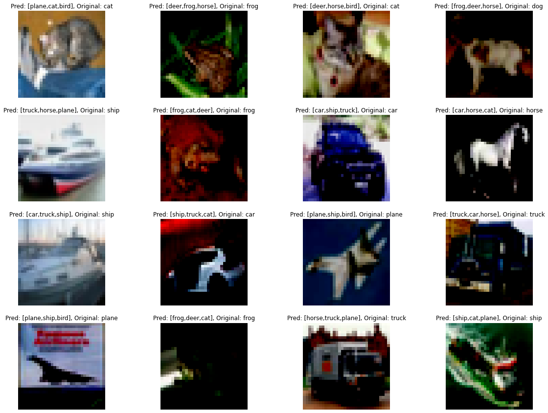
Training this model on CIFAR 10 dataset for 10 epochs resulted in a decent performance. Following are the results of the test set.

Conclusion

Involution is a super good primitive block that can outperform convolution block in many vision-related tasks. It can even compete with self-attention and achieve SOTA results. It is easy to implement, scales well, and robust. We can potentially see more architectures using this block in the near future.

References

Involution Paper

Original Implementation

Colab NoteBook

Convolutional kernels

Convolution Image Source

ResNet Image Source

Feature Image by @quinguyen

My Linkedin Profile