One of the fastest-growing areas of technology is machine learning, but even seasoned professionals occasionally stumble over new terms and jargon. It is simple to get overwhelmed by the plethora of technical terms as research speeds up and new architectures, loss functions, and optimisation techniques appear.
This blog article is your carefully chosen reference to more than fifty key and sophisticated machine learning terms. Some of these are widely recognised, while others are rarely defined but have a significant impact. With clear explanations and relatable examples, we dissect everything from fundamental ideas like overfitting and bias-variance tradeoff to innovative ideas like LoRA, Contrastive Loss, and One Cycle Policy.
So, dive in and surprise yourself with how many of these machine learning terms you didn’t fully grasp until now.
Model Training & Optimization
Foundational machine learning terms that enhance model efficiency, stability, and convergence during training.
1. Curriculum Learning
A training approach in which more complex examples are progressively added to the model after it has been exposed to simpler ones. This can enhance convergence and generalisation by mimicking human learning.
Example: Before introducing noisy, low-quality images, a digit classifier is trained on clear, high-contrast images.
It’s similar to teaching a child to read, by having them start with basic three-letter words before progressing to more complicated sentences and paragraphs. This method keeps the model from becoming disheartened or stuck on challenging problems in the early stages of training. The model can more successfully handle more difficult problems later on by laying a strong foundation on simple ideas.
2. One Cycle Policy
A learning rate schedule that boosts convergence and training efficiency by starting small, increasing to a peak, and then decreasing again.
Example: The learning rate varies from 0.001 to 0.01 to 0.001 over different epochs.
This approach is similar to giving your model a “warm-up, sprint, and cool-down.” The model can get its bearings with the low learning rate at the beginning, learn quickly and bypass suboptimal regions with the high rate in the middle, and fine-tune its weights and settle into a precise minimum with the final decrease. Models are frequently trained more quickly and with greater final accuracy using this cycle.
3. Lookahead Optimizer
Smoothes the optimisation path by wrapping around current optimisers and keeping slow-moving weights updated based on the direction of the fast optimiser.
Example: Lookahead + Adam results in more rapid and steady convergence.
Consider this as having a “main army” (the slow weights) that follows the general direction the scout finds and a quick “scout” (the inner optimiser) that investigates the terrain ahead. The army follows a more stable, direct route, but the scout may zigzag. The model converges more consistently and the variance is decreased with this dual-speed method.
4. Sharpness Aware Minimization (SAM)
An optimisation method that promotes models to converge to flatter minima, which are thought to be more applicable to data that hasn’t been seen yet.
Example: Results in stronger models that function well with both test and training data.
Consider attempting to keep a ball balanced in a valley. A broad, level basin (a flat minimum) is far more stable than a narrow, sharp canyon (a sharp minimum). During training, SAM actively looks for these broad basins, creating more resilient models because minor adjustments to the input data won’t cause the valley to collapse.
5. Gradient Clipping
Stops the gradients from blowing up (growing too big) by capping them at a specific value. In recurrent networks in particular, this guarantees stable training.
Example: To avoid divergence during training, RNN gradients are clipped.
Consider capping the volume of a shout. The model’s reaction (the gradient) is kept within a reasonable range regardless of how unexpected an error is. This stops the model from updating its weights in a huge, unstable way, which is known as “exploding gradients” and can totally ruin the training process.
6. Bayesian Optimization
A technique for optimising functions that are costly to evaluate (such as hyperparameter tuning) by directing the search with probabilistic models.
Example: Use fewer training runs to effectively determine the optimal learning rate.
When every trial run is extremely costly and slow, this is a clever search method for determining the ideal model settings. Based on the trials it has already conducted, it creates a probabilistic “map” of how it believes various settings will function. It then makes an informed decision about where to search next using this map, concentrating on areas that show promise and avoiding wasting time on settings that it believes will perform poorly.
Read about Bayesian Thinking in detail here.
7. Batch Renormalization
A variation of batch normalisation that fixes differences between batch and global statistics, making it more stable when small batch sizes are used.
Example: Assists in training models when the batch size is limited to 4 by GPU memory.
When batch normalisation can view a sizable, representative collection of examples at once, it performs at its best. Batch Renormalisation serves as a corrective lens when you can only use a small batch, modifying the statistics from the small group to more closely resemble the appearance of the entire dataset. When you are forced to use small batches due to hardware limitations, this helps stabilize training.
Regularization & Generalization
These are machine learning terms that help models generalise better to unseen data while avoiding overfitting and memorisation.
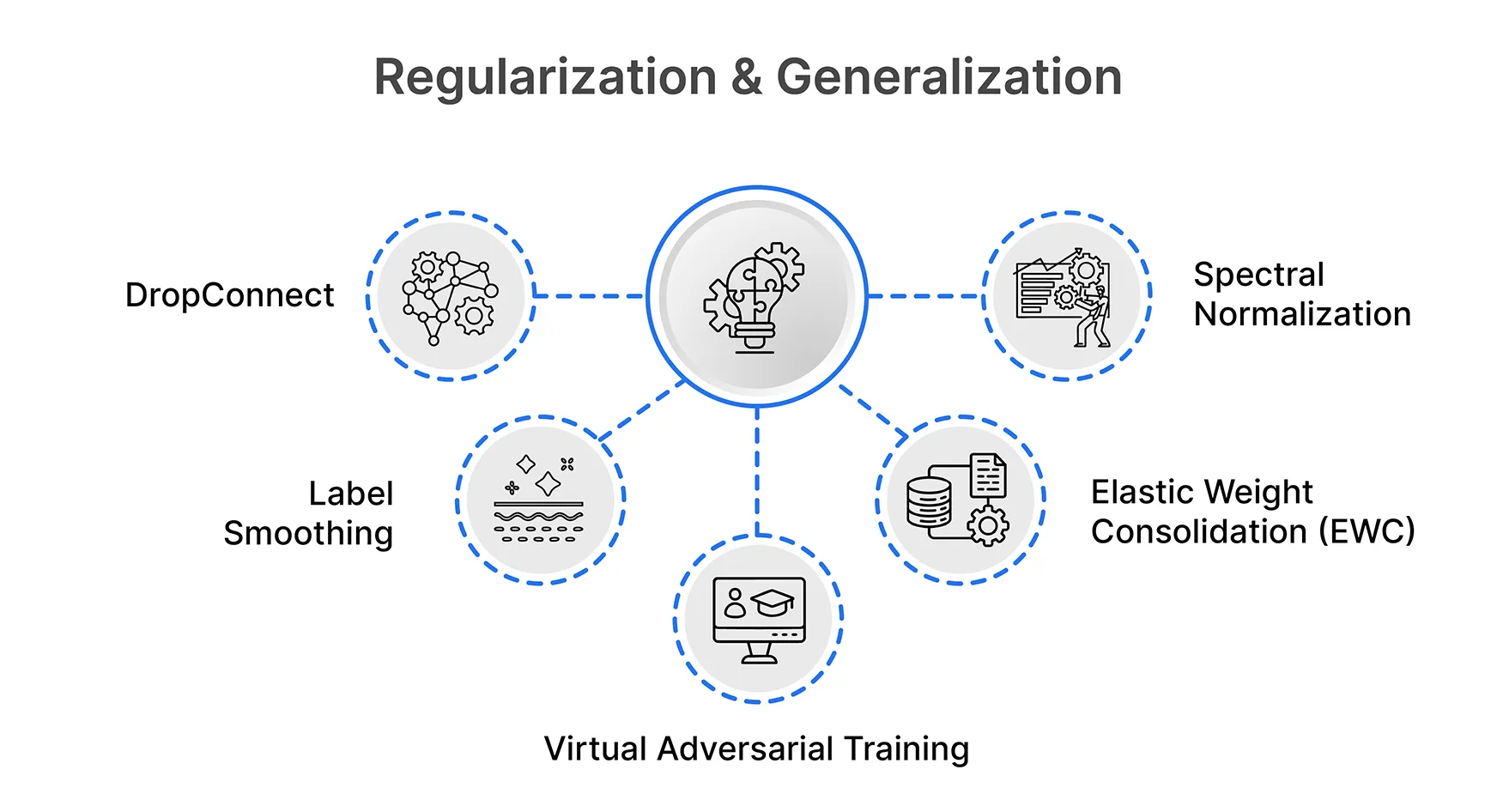
8. DropConnect
Instead of dropping entire neurons during training, as in Dropout, this regularisation technique randomly drops individual weights or connections between neurons.
Example: A weight between two neurons is disabled during training, introducing robustness.
By deactivating individual connections, DropConnect provides a more granular method than the widely used Dropout technique, which momentarily deactivates entire neurons. Consider a social network in which DropConnect is similar to randomly cutting individual phone lines between users, while Dropout is similar to telling specific users to be silent. This keeps the network from becoming overly dependent on any one connection and forces it to create more redundant pathways.
9. Label Smoothing
A method of softening the labels during training to keep the model from growing overconfident. It gives the wrong classes a tiny portion of the probability mass.
Example: Class A should be labelled 0.9 rather than 1.0, and the others should be labelled 0.1.
The model learns a little humility from this approach. You ask it to be 99% certain about a prediction, acknowledging the very small possibility that it might be incorrect, rather than expecting it to be 100% certain. In addition to improving the model’s calibration and adaptability to novel, unseen examples, this stops the model from making wildly optimistic predictions.
10. Virtual Adversarial Training
Adds tiny changes to inputs during training to regularise predictions, increasing the robustness of the model.
Example: To improve classification stability, add subtle noise to images.
This method works similarly to a sparring partner who continuously nudges you in your weak areas to strengthen you. The model is trained to be resistant to that particular change after determining which direction a small change in the input would most likely affect the model’s prediction. As a result, the model is more reliable and less susceptible to being tricked by erratic or noisy real-world data.
11. Elastic Weight Consolidation (EWC)
A regularisation technique that penalises significant weights from changing excessively in order to maintain knowledge of prior tasks.
Example: As you learn new tasks, you don’t forget old ones.
Consider a person who has mastered the guitar and is now learning to play the piano. By recognising the essential “muscle memory” (important weights) from the guitar task, EWC serves as a memory aid. It makes switching between those particular weights more difficult when l8809earning the piano, maintaining the old skill while enabling the acquisition of new ones.
12. Spectral Normalization
A method to increase training stability in neural networks by constraining the spectral norm of weight matrices.
Example: Lipschitz constraints are applied in GAN discriminators to provide more stable adversarial training.
Consider this as setting limits on how quickly your model can alter its behaviour. Spectral normalisation keeps the training from becoming chaotic or unstable by regulating the “maximum amplification” that each layer can apply.
Model Architectures & Components
This section introduces advanced machine learning terms related to how neural networks are structured and how they process information.
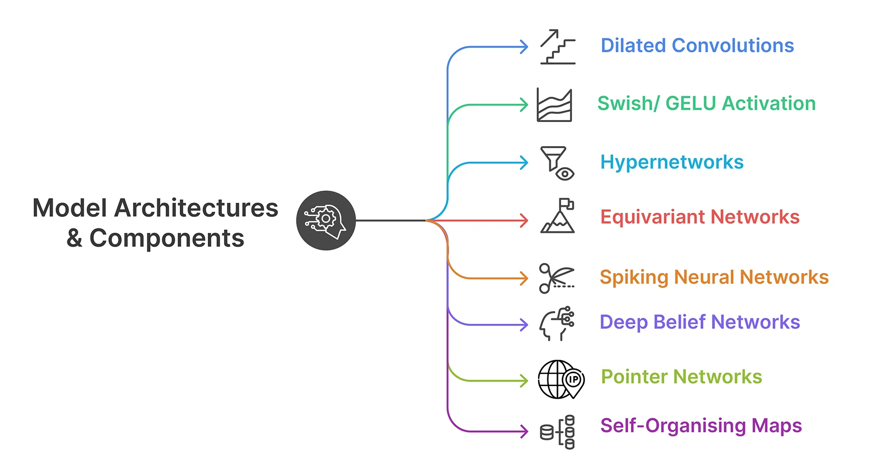
13. Dilated Convolutions
Networks can have a wider receptive field without adding more parameters thanks to convolution operations that create gaps (dilations) between kernel elements.
Example: WaveNet is used in audio generation to record long-range dependencies.
This is similar to having a network that doesn’t require larger eyes or ears to “see” a larger portion of an image or “hear” a longer audio clip. The convolution can capture more context and cover more ground with the same computational cost by spreading out its kernel. It’s similar to taking larger steps to gain a quicker understanding of the big picture.
14. Swish/ GELU Activation
Smoother and more differentiable than ReLU, advanced activation functions help in convergence and performance in deeper models.
Example: EfficientNet uses Swish for increased accuracy, while BERT uses GELU.
Swish and GELU are similar to dimmer switches if ReLU is a basic on/off light switch. In contrast to ReLU’s sharp corner, their smooth curves facilitate gradient flow during backpropagation, which stabilises the training process. This minor adjustment facilitates more fluid information processing, which frequently improves final accuracy.
15. Hypernetworks
Dynamic and conditional model architectures are made possible by neural networks that produce the weights of other neural networks.
Example: MetaNet creates layer weights for various tasks dynamically.
Consider a “master network” that serves as a factory, producing the weights for a distinct “worker network,” rather than solving problems on its own. This enables you to quickly develop customised worker models that are suited to particular tasks or inputs. It’s an effective method for increasing the adaptability and flexibility of models.
16. Equivariant Networks
Predictive networks that preserve symmetry properties (such as translation or rotation) are helpful in scientific fields.
Example: Rotation-equivariant CNNs are employed in medical imaging and 3D object recognition.
The architecture of these networks incorporates fundamental symmetries, such as the laws of physics. For example, a rotation-equivariant network will not alter its prediction because it understands that a molecule remains the same even when it is rotated in space. For scientific data where these symmetries are essential, this makes them extremely accurate and efficient.
17. Spiking Neural Networks
This kind of neural network transmits information using discrete events (spikes) rather than continuous values, more like biological neurons.
Example: It is utilised in energy-efficient hardware for applications such as real-time sensory processing.
Similar to how our own neurons fire, SNNs communicate in brief, sharp bursts rather than in a continuous hum of information.
18. Deep Belief Networks
A class of deep neural network, or generative graphical model, is made up of several layers of latent variables (also known as “hidden units”), with connections between the layers but not between units within each layer.
Example: Deep neural networks are pre-trained using this method.
It resembles a stack of pancakes, with each pancake standing for a distinct degree of data abstraction.
19. Pointer Networks
A particular kind of neural network that can be trained to identify a particular sequence element.
Example: Applied to solve issues such as the travelling salesman problem, in which determining the quickest path between a group of cities is the aim.
Comparable to having a GPS that can indicate the next turn at every intersection is this analogy.
20. Self-Organising Maps
A kind of unsupervised neural network that creates a discretised, low-dimensional representation of the training samples’ input space.
Example: Used to display high-dimensional data in a way that makes its underlying structure visible.
It’s similar to assembling a set of tiles into a mosaic, where each tile stands for a distinct aspect of the original picture.
Data Handling & Augmentation
Learn machine learning terms focused on preparing, managing, and enriching training data to boost model performance.
21. Mixup Training
An approach to data augmentation that smoothes the decision boundaries and lessens overfitting by interpolating two images and their labels to produce synthetic training samples.
Example: A new image with a label that reflects the same mix is made up of 70% dog and 30% cat.
By using this method, the model learns that things aren’t always black and white. The model learns to make less certain predictions and foster a more seamless transition between categories by being shown blended examples. This keeps the model from overestimating itself and improves its ability to generalise to new, potentially ambiguous data.
22. Feature Store
A centralised system for team and project management, ML feature serving, and reuse.
Example: Save and utilise the “user age bucket” for various models.
Consider a feature store as a high-quality, communal pantry for data scientists. They can pull reliable, pre-processed, and documented features from the central store rather than having each cook (data scientist) make their own ingredients (features) from scratch for each meal (model). This guarantees uniformity throughout an organisation, minimises errors, and saves a ton of redundant work.
23. Batch Effect
Systematic technical differences that can confuse analysis results between batches of data.
Example: Gene expression data processed on various days reveals consistent variations unrelated to biology.
Imagine this as multiple photographers taking pictures of the same scene with different cameras. Technical variations in equipment produce systematic variations that require correction, even though the subject is the same.
Evaluation, Interpretability, & Explainability
These machine learning terms help quantify model accuracy and provide insights into how and why predictions are made.
24. Cohen’s Kappa
A statistical metric that takes into consideration the possibility of two classifiers or raters agreeing by chance.
Example: Kappa accounts for random agreement and may be lower even if two doctors agree 85% of the time.
This metric assesses “true agreement” beyond what would be predicted by chance alone. Two models will have high raw agreement if they both classify 90% of items as “Class A,” but Kappa corrects for the fact that they would have agreed greatly if they had simply consistently guessed “Class A.” “How much are the raters truly in sync, beyond random chance?” is the question it addresses.
25. Brier Score
Calculates the mean squared difference between expected probabilities and actual results to assess how accurate probabilistic predictions are.
Example: A model with more accurately calibrated probabilities will score lower on the Brier scale.
This score evaluates a forecaster’s long-term dependability. A high Brier score indicates that, on average, rain fell roughly 70% of the time when a weather model predicted a 70% chance of rain. It incentivises truthfulness and precision in probability calculations.
26. Counterfactual Explanations
Explain how a different model prediction could result from altering the input features.
Example: A user’s loan would be granted if their income was $50,000 rather than $30,000.
This approach provides an explanation of a decision by answering the “what if” question. It offers a tangible, doable alternative rather than merely stating the result. “Your loan would have been approved if your down payment had been $5,000 higher,” it might state in response to a denied loan application. The logic of the model becomes clear and intelligible as a result.
27. Anchors
High-precision, straightforward rules that, in some circumstances, ensure a prediction.
Example: “Always approve a loan if the borrower is older than 60 and earns more than $80,000.”
Anchors give a model’s prediction a “safe zone” of clear, uncomplicated rules. They pinpoint a narrow range of circumstances in which the model behaves in a fixed and predictable manner. Despite the complexity of the model’s overall behaviour, this offers a precise, highly reliable explanation for why a particular prediction was made.
28. Integrated Gradients
An attribution technique that integrates gradients along the input path to determine the corresponding contribution of each input feature to a prediction.
Example: Indicates which pixels had the greatest impact on an image’s classification. Somewhat similar to what GradCAM does.
In essence, this method produces a “heat map” of the input features’ relative importance. It identifies the precise pixels that the model “looked at” in order to classify an image, such as a cat’s whiskers and pointed ears. It can reveal the words that had the biggest impact on the sentiment of a text decision.
29. Out of Distribution Detection
Finding inputs that differ from the data used to train a model.
Example: The camera system of a self-driving car should be able to recognise when it is seeing an entirely different kind of object that it has never seen before.
An analogy would be a quality control inspector on an assembly line searching for goods that are entirely different from what they should be.
Continual & Lifelong Learning
This part explains machine learning terms relevant to models that adapt over time without forgetting previously learned tasks.
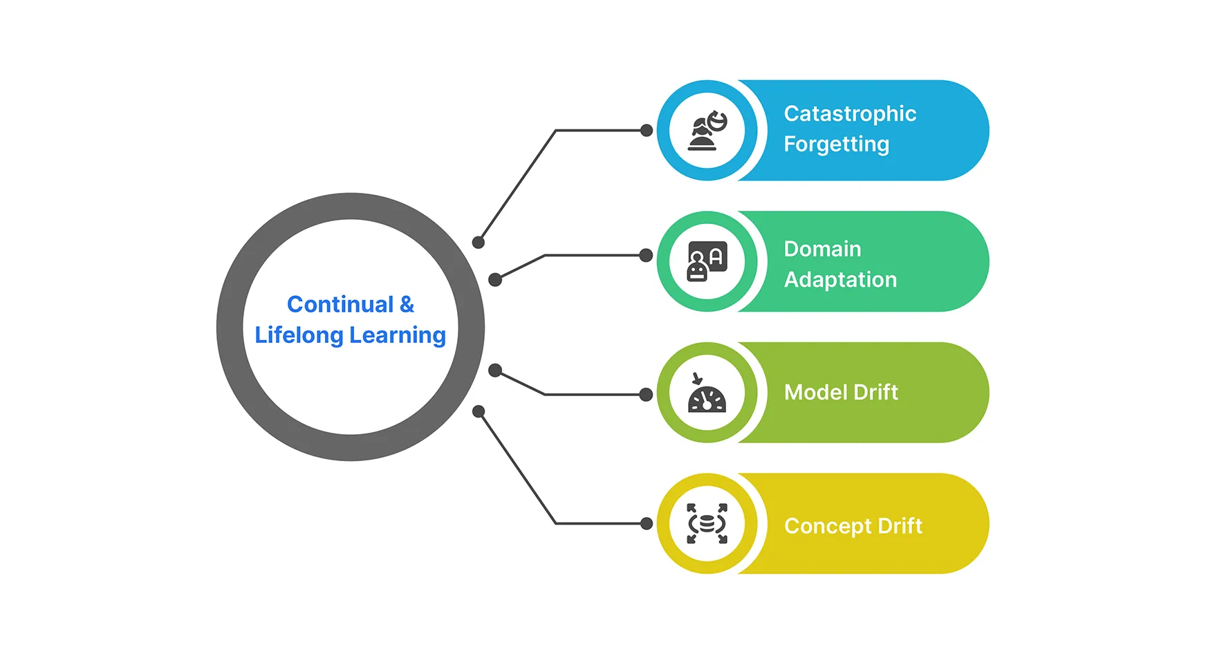
30. Catastrophic Forgetting
A situation where a model is trained on new tasks and then forgets what it has already learnt. This is a significant obstacle to lifelong learning and is particularly common in sequential learning.
Example: After being retrained to recognise vehicles, a model that was trained to recognise animals completely forgets them.
This occurs as a result of the model replacing the network weights that held the previous data with the new weights required for the new task. It’s comparable to how someone who has spoken only their native tongue for years may forget a language they learnt in high school. Developing AI that can continuously learn new things without requiring retraining on everything it has ever seen is extremely difficult.
31. Domain Adaptation
The challenge of adapting a model trained on a source data distribution to a different but related target data distribution is addressed in this area of machine learning.
Example: It might be necessary to modify a spam filter that was trained on emails from one organisation in order for it to function properly on emails from another.
An analogy would be a translator who speaks one dialect of a language well but needs to learn another.
32. Model Drift
Occurs when a model’s performance deteriorates over time as a result of shifting input data distributions.
Example: E-commerce recommender models are impacted by changes in consumer behaviour following the COVID-19 pandemic.
At this point, a once-accurate model loses its relevance because the environment it was trained in has evolved. It’s similar to trying to navigate a city in 2025 using a map from 2019; while the map is accurate, new roads have been constructed and old ones have been closed. To stay up to date, production models need to be continuously checked for drift and retrained using fresh data.
33. Concept Drift
This phenomenon occurs when the target variable’s statistical characteristics, which the model is attempting to forecast, alter over time in unexpected ways.
Example: As customer behaviour evolves over time, a model that forecasts customer attrition may lose accuracy.
An analogy would be attempting to navigate a city using an outdated map. The map may no longer be as helpful because the streets and landmarks have changed.
Loss Functions & Distance Metrics
These machine learning terms define how model predictions are evaluated and compared to actual outcomes.
34. Contrastive Learning
Pushes dissimilar data apart and encourages representations of similar data to be closer together in latent space.
Example: SimCLR compares pairs of augmented images to learn representations. CLIP also makes use of this logic.
This functions similarly to an AI “spot the difference” game. An image (the “anchor”), a slightly modified version of it (the “positive”), and an entirely different image (the “negative”) are presented to the model. Its goal is to learn to pull the anchor and positive closer together while pushing the negative far away, effectively learning what makes an image unique.
35. Triplet Loss
In order to train models to embed similar inputs closer together and dissimilar inputs farther apart in a learnt space, a loss function is utilised.
Example: A face recognition system’s model is trained to maximise the distance between two images of the same person and maximise the distance between two images of different people.
Putting books by the same author next to each other and books by different authors on different shelves is analogous to arranging your bookshelf.
36. Wasserstein Distance
More significant distances than KL divergence are provided by a metric that calculates the “cost” of changing one probability distribution into another.
Example: Wasserstein GANs use it to give training gradients greater stability.
Consider this to be the least amount of work required to move one sand pile to match the shape of another. The “transport cost” of moving probability mass around is taken into account by the Wasserstein distance, in contrast to other distance measures.
Advanced Concepts & Theory
These are high-level machine learning terms that underpin cutting-edge research and theoretical breakthroughs.
37. Lottery Ticket Hypothesis
Proposes that there is a smaller, properly initialised subnet (a “winning ticket”) inside a larger, overparameterized neural network that can be trained separately to achieve similar performance.
Example: High accuracy can be achieved by training a small portion of a pruned ResNet50 from scratch.
Imagine a massive, randomly distributed network as a massive lottery pool. According to the hypothesis, a small, flawlessly organised sub-network the “winning ticket” has been concealed from the start. Finding this unique subnet will allow you to save a ton of computation by training just that subnet and getting the same fantastic results as training the entire massive network. The biggest obstacle, though, is coming up with a practical way to locate this “winning ticket.”
38. Meta Learning
This process, sometimes referred to as “learning to learn,” involves teaching a model to rapidly adjust to new tasks with little data.
Example: MAML makes it possible to quickly adjust to novel image recognition tasks.
The model learns the general process of learning rather than a single task. It’s similar to teaching a student to learn extremely quickly so that they can master a new subject (task) with minimal study materials (data). To achieve this, the model is trained on a broad range of learning tasks.
39. Neural Tangent Kernel
A theoretical framework that offers insights into generalisation by examining the learning dynamics of infinitely wide neural networks.
Example: It facilitates the analysis of deep networks’ training behaviour in the absence of actual training.
NTK is a powerful mathematical tool that links deep learning to more traditional, well-understood kernel techniques. It enables researchers to make accurate theoretical claims about the learning process of very wide neural networks and the reasons behind their generalisation to new data. It offers a quick way to comprehend the dynamics of deep learning without requiring costly training experiments.
40. Manifold Learning
Finding a low-dimensional representation of high-dimensional data while maintaining the data’s geometric structure is the goal of this class of unsupervised learning algorithms.
Example: To gain a better understanding of the structure of a high-dimensional dataset, visualize it in two or three dimensions.
It’s like creating a flat map of the Earth. You’re representing a three-dimensional object in two dimensions, but you’re trying to preserve the relative distances and shapes of the continents.
41. Disentagled Representation
A kind of representation learning in which the features that are learnt match unique, comprehensible factors of variation in the data.
Example: A model that learns to depict faces may have distinct features for facial expression, eye colour, and hair colour.
Comparable to a set of sliders, it allows you to adjust various aspects of an image, including its saturation, contrast, and brightness.
42. Gumbel-Softmax Trick
Gradient-based optimisation using discrete choices is made possible by this differentiable approximation of sampling from a categorical distribution.
Example: Variational autoencoders are trained end-to-end using categorical latent variables in discrete latent variable models. Getting a “soft gradient” that you can still train through is similar to rolling a weighted dice.
This technique produces a smooth approximation that appears discrete but is still differentiable, allowing backpropagation through sampling operations, as opposed to making difficult discrete decisions that block gradients.
43. Denoising Score Matching
A method for estimating the gradient of the log-density (score function) through model training in order to learn probability distributions.
Example: Score matching is used by diffusion models to learn how to reverse the noise process and produce new samples.
This is similar to learning how to “push” each pixel in the right direction to make a messy image cleaner. You learn the gradient field pointing towards higher probability regions rather than directly modelling probabilities.
Deployment & Production
This section focuses on machine learning terms that ensure models run efficiently, reliably, and safely in real-world environments.
44. Shadow Deployment
An approach used for silent testing in which a new model is implemented concurrently with the existing one without affecting end users.
Example: Risk-free model quality testing in production.
Having a trainee pilot fly a plane in a simulator that receives real-time flight data but whose actions don’t actually control the aircraft is analogous to this. You can test the new model’s performance on real-world data without endangering users because the system can record its predictions and compare them to the decisions made by the live model.
45. Serving Latency
Serving Latency is how long it takes for a model that has been deployed to produce a prediction. In real-time systems, low latency is essential.
Also read: From 10s to 2s: Complete p95 Latency Reduction Roadmap Using Cloud Run and Redis
Example: A voice assistant needs a model response of less than 50 ms.
This is the amount of time that passes between posing a query to the model and getting a response. Speed is just as crucial as accuracy in many real-world applications, like language translation, online ad bidding, and fraud detection. Low latency is a crucial prerequisite for deployment since a prediction that comes too late is frequently worthless.
Probabilistic & Generative Methods
Explore machine learning terms that deal with uncertainty modelling and the generation of new, data-like samples through probabilistic techniques.
46. Variational Inferences
An approximate technique that uses optimization over distributions instead of sampling to carry out Bayesian inference.
Example: A probabilistic latent space is learnt in VAEs.
For probability problems that are too difficult to compute precisely, this is a useful mathematical shortcut. Rather than attempting to determine the precise, intricate form of the actual probability distribution, it determines that the best approximation is a simpler, easier-to-manage distribution (such as a bell curve). This transforms an unsolvable computation into a manageable optimisation issue.
47. Monte Carlo Dropout
A method for estimating prediction uncertainty that involves averaging predictions over several forward passes and applying dropout at inference time.
Example: To obtain uncertainty estimates, make several predictions about the tumour probability.
By maintaining dropout, which is typically only active during training, at prediction time, this method transforms a standard network into a probabilistic one. You can obtain a variety of marginally different outputs by passing the same input through the model 30 or 50 times. You can get a reliable estimate of the model’s prediction uncertainty from the distribution of these outputs.
48. Knowledge Distillation
A compression method that uses softened outputs to teach a smaller “student” model to imitate a larger “teacher” model.
Example: Rather than using hard labels, the student learns from soft class probabilities.
Consider an apprentice (the small student model) being taught by a master craftsman (the large teacher model). In addition to displaying the final right response, the master provides a detailed “why” (e.g., “this looks 80% like a dog, but it has some cat-like features”). The soft probabilities’ additional information greatly supports the smaller student model in learning the same intricate reasoning.
You can read all about Distilled Models here.
49. Normalizing Flows
To convert a simple probability distribution into a complex one for generative modelling, use a series of invertible functions.
Example: Glow creates excellent images by using normalising flows.
Consider these as a set of mathematical prisms that can stretch, bend, and twist a basic shape, such as a homogeneous blob of clay, into a highly intricate sculpture, such as the distribution of faces in the real world, by applying a series of reversible transformations. They can be used to determine the precise probability of existing data as well as to create new data because each step is completely reversible.
50. Causal Inference
A branch of machine learning and statistics that focuses on figuring out the causal relationships between variables.
Example: Figuring out if a new marketing campaign genuinely increased sales or if it was merely a coincidence.
The difference between understanding that roosters crow when the sun rises and understanding that the sun does not rise as a result of the rooster’s crow is analogous.
51. Dynamic Time Warping
An algorithm that finds the best alignment between temporal sequences that might differ in timing or speed in order to measure similarity.
Example: Comparing two speech signals with varying speeds or matching up financial time series with various seasonal trends.
Similar to matching the notes of two songs sung at different tempos. You can compare sequences even when timing differs greatly because DTW compresses and stretches the time axis to find the optimal alignment.
Conclusion
It takes more than just learning definitions to comprehend these 50+ machine learning terms; it also requires developing an understanding of how contemporary ML systems are developed, trained, optimized, and implemented.
These concepts highlight the intricacy and beauty of the systems we deal with on a daily basis, from how models learn (One Cycle Policy, Curriculum Learning), how they generalize (Label Smoothing, Data Augmentation), and even how they behave badly (Data Leakage, Mode Collapse).
Whether you’re reading a research paper, developing your next model, or troubleshooting unexpected outcomes, let this glossary of machine learning terms serve as a mental road map to help you navigate the constantly changing field.
GenAI Intern @ Analytics Vidhya | Final Year @ VIT Chennai
Passionate about AI and machine learning, I'm eager to dive into roles as an AI/ML Engineer or Data Scientist where I can make a real impact. With a knack for quick learning and a love for teamwork, I'm excited to bring innovative solutions and cutting-edge advancements to the table. My curiosity drives me to explore AI across various fields and take the initiative to delve into data engineering, ensuring I stay ahead and deliver impactful projects.