Deep Learning for Image Super-Resolution

Introduction

 

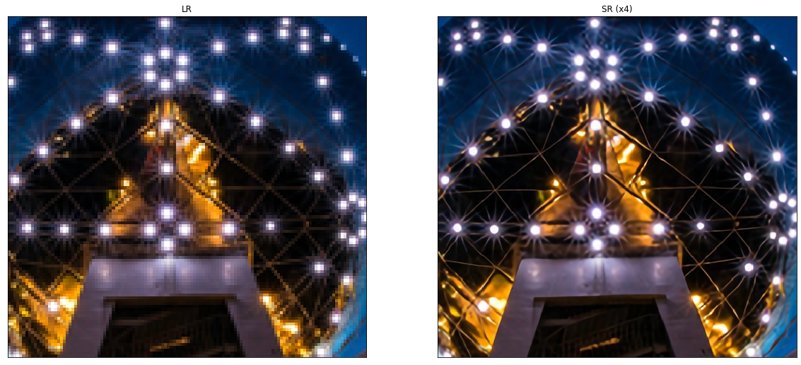
Image super-resolution (SR) is the process of recovering high-resolution (HR) images from low-resolution (LR) images. It is an important class of image processing techniques in computer vision and image processing and enjoys a wide range of real-world applications, such as medical imaging, satellite imaging, surveillance and security, astronomical imaging, amongst others.

With the advancement in deep learning techniques in recent years, deep learning-based SR models have been actively explored and often achieve state-of-the-art performance on various benchmarks of SR. A variety of deep learning methods have been applied to solve SR tasks, ranging from the early Convolutional Neural Networks (CNN) based method to recent promising Generative Adversarial Nets based SR approaches.

Problem

Image super-resolution (SR) problem, particularly single image super-resolution (SISR), has gained a lot of attention in the research community. SISR aims to reconstruct a high-resolution image I^SR from a single low-resolution image I^LR. Generally, the relationship between I^LR and the original high-resolution image I^HR can vary depending on the situation. Many studies assume that I^LR is a bicubic downsampled version of I^HR, but other degrading factors such as blur, decimation, or noise can also be considered for practical applications.

In this article, we would be focusing on supervised learning methods for super-resolution tasks. By using HR images as target and LR images as input, we can treat this problem as a supervised learning problem.

Upsampling Methods

Before understanding the rest of the theory behind the super-resolution, we need to understand upsampling (Increasing the spatial resolution of images or simply increasing the number of pixel rows/columns or both in the image) and its various methods.

1. Interpolation-based methods – Image interpolation (image scaling), refers to resizing digital images and is widely used by image-related applications. The traditional methods include nearest-neighbor interpolation, linear, bilinear, bicubic interpolation, etc.

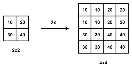
Nearest-neighbor interpolation with the scale of 2

• Nearest-neighbor Interpolation – The nearest-neighbor interpolation is a simple and intuitive algorithm. It selects the value of the nearest pixel for each position to be interpolated regardless of any other pixels.
• Bilinear Interpolation – The bilinear interpolation (BLI) first performs linear interpolation on one axis of the image and then performs on the other axis. Since it results in a quadratic interpolation with a receptive field-sized 2 × 2, it shows much better performance than nearest-neighbor interpolation while keeping a relatively fast speed.
• Bicubic Interpolation – Similarly, the bicubic interpolation (BCI) performs cubic interpolation on each of the two axes Compared to BLI, the BCI takes 4 × 4 pixels into account, and results in smoother results with fewer artifacts but much lower speed. Refer to this for a detailed discussion.

Shortcomings – Interpolation-based methods often introduce some side effects such as computational complexity, noise amplification, blurring results, etc.

2. Learning-based upsampling – To overcome the shortcomings of interpolation-based methods and learn upsampling in an end-to-end manner, transposed convolution layer and sub-pixel layer are introduced into the SR field.

 

Transposed convolution layer  –  The blue boxes denote the input,
and the green boxes indicate the kernel and the convolution output.

• Transposed convolution: layer, a.k.a. deconvolution layer, tries to perform transformation opposite a normal convolution, i.e., predicting the possible input based on feature maps sized like convolution output. Specifically, it increases the image resolution by expanding the image by inserting zeros and performing convolution.

Sub-pixel layer – The blue boxes denote the input and the boxes with other colors indicate different convolution operations and different output feature maps.

• Sub-pixel Layer: The sub-pixel layer, another end-to-end learnable upsampling layer, performs upsampling by generating a plurality of channels by convolution and then reshaping them shows. Within this layer, a convolution is firstly applied for producing outputs with
  s² times channels, where s is the scaling factor. Assuming the input size is h × w × c, the output size will be h×w×s²c. After that, the reshaping operation is performed to produce outputs with size sh × sw × c

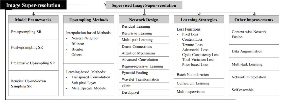
Super-resolution Frameworks

Since image super-resolution is an ill-posed problem, how to perform upsampling (i.e., generating HR output from LR input) is the key problem. There are mainly four model frameworks based on the employed upsampling operations and their locations in the model (refer to the table above).

1. Pre-upsampling Super-resolution –

 

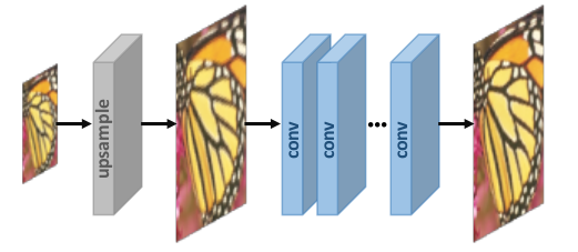
We don’t do a direct mapping of LR images to HR images since it is considered to be a difficult task. We utilize traditional upsampling algorithms to obtain higher resolution images and then refining them using deep neural networks is a straightforward solution. For example – LR images are upsampled to coarse HR images with the desired size using bicubic interpolation. Then deep CNNs are applied to these images for reconstructing high-quality images.

2. Post-upsampling Super-resolution –

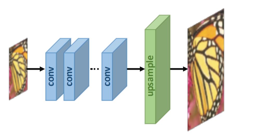
To improve the computational efficiency and make full use of deep learning technology to increase resolution automatically, researchers propose to perform most computation in low-dimensional space by replacing the predefined upsampling with end-to-end learnable layers integrated at the end of the models. In the pioneer works of this framework, namely post-upsampling SR, the LR input images are fed into deep CNNs without increasing resolution, and end-to-end learnable upsampling layers are applied at the end of the network.

Learning Strategies

In the super-resolution field, loss functions are used to
measure reconstruction error and guide the model optimization. In early times, researchers usually employ the pixelwise L2 loss(mean squared error), but later discover that it cannot measure the
reconstruction quality very accurately. Therefore, a variety
of loss functions (e.g., content loss, adversarial loss) are adopted for better measuring the reconstruction
error and producing more realistic and higher-quality results.

• Pixelwise L1 loss – Absolute difference between pixels of ground truth HR image and the generated one.
• Pixelwise L2 loss – Mean squared difference between pixels of ground truth HR image and the generated one.
• Content loss – the content loss is indicated as the Euclidean distance between high-level representations of the output image and the target image. High-level features are obtained by passing through pre-trained CNNs like VGG and ResNet.
• Adversarial loss – Based on GAN where we treat the SR model as a generator, and define an extra discriminator to judge whether the input image is generated or not.
• PSNR – Peak Signal-to-Noise Ratio (PSNR) is a commonly used objective metric to measure the reconstruction quality of a lossy transformation. PSNR is inversely proportional to the logarithm of the Mean Squared Error (MSE) between the ground truth image and the generated image.

In MSE, I is a noise-free m×n monochrome image (ground truth)  and K is the generated image (noisy approximation). In PSNR, MAX_I represents the maximum possible pixel value of the image.

Network Design

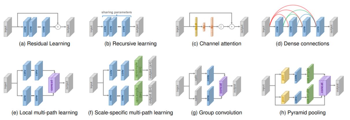
Various network designs in super-resolution architecture

Enough of the basics! Let’s discuss some of the state-of-art super-resolution methods –

Super-Resolution methods

Super-Resolution Generative Adversarial Network (SRGAN) – Uses the idea of GAN for super-resolution task i.e. generator will try to produce an image from noise which will be judged by the discriminator. Both will keep training so that generator can generate images that can match the true training data.

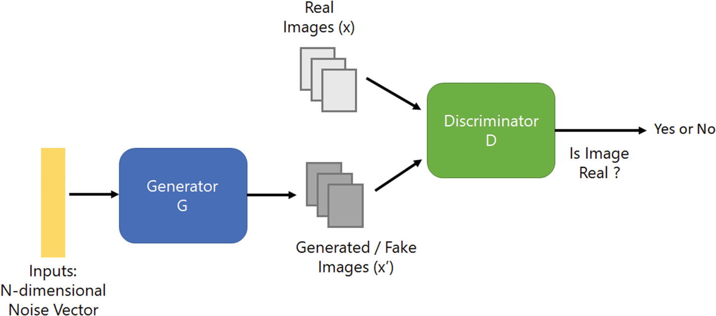
Architecture of Generative Adversarial Network

Check the original papers for detailed information.

Steps –

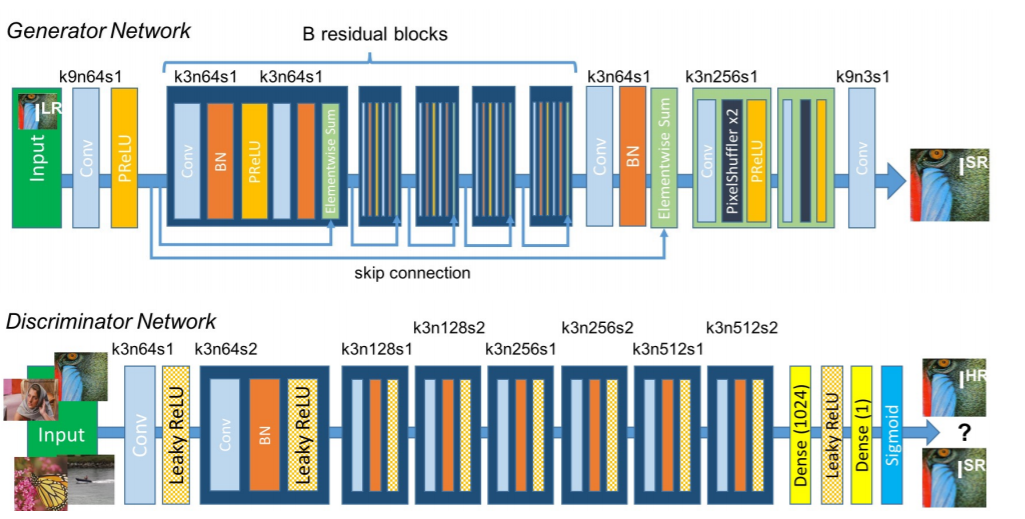
Network architecture of SRGAN

Key features of the method – 

EDSR, MDSR – Residual learning techniques exhibit
improved performance of super-resolution through deep convolutional neural networks(DCNN). Single-scale architecture Enhanced Deep Super-Resolution network(EDSR) handles specific super-resolution scale and Multi-scale Deep Super-Resolution system(MDSR) reconstructs various scales of high-resolution images in a single model. The significant performance improvement of the model
is due to optimization by removing unnecessary modules in
conventional residual networks.

Check the original papers for detailed information.

Some of the key features of the methods – 

• Residual blocks – SRGAN successfully applied the ResNet architecture to the super-resolution problem with SRResNet, they further improved the performance by employing a better ResNet structure. In the proposed architecture –

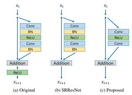
Comparison of the residual blocks

• They removed the batch normalization layers from the network as in SRResNets. Since batch normalization layers normalize the features, they get rid of range flexibility from networks by normalizing the features, it is better to remove them.

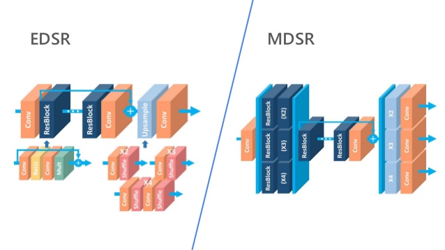
• In MDSR, they proposed a multiscale architecture that shares most of the parameters on different scales. The proposed multiscale model uses significantly fewer parameters than multiple single-scale models but shows comparable performance.

Original code of the methods

So now we have come to the end of the blog! To learn about super-resolution, refer to these survey papers.

Kindly share your feedback about the blog in the comment section. Happy Learning 🙂