An Intuitive Way to Understand Gradient Descent with Some Python Code

This article was published as a part of the Data Science Blogathon

Introduction

“There is a saying ‘A jack of all trades and a master of none.’ When it comes to being a data scientist you need to be a bit like this, but perhaps a better saying would be, ‘A jack of all trades and a master of some.’” ―Brendan Tierney, Principal Consultant at Oralytics

If we look up searches on the web on maths related to Data Science, three topics that pop up quite frequently are Calculus, Linear Algebra and Statistics. As a Data Scientist, a solid fundamental grasp of mathematics under the hood helps when we are implementing our model. This article is an attempt to present in a lucid manner,  one such important data science concept which involves understanding mathematics.

When we are building a Machine Learning model for a real-life dataset, there are two terms that we encounter. One is Objective Function and the other is the Optimization Algorithm. Let’s try and understand these two jargons closely. In the case of supervised machine learning (labelled training data), the model predicts an output and which we compare against a reference actual value which we can call Target. The Objective Function provides an insight to the Data Scientist as to how well the output predicted by the model match the desired output values. This is a sort of reality check on our model performance. Another term we use for this is Loss Function or Cost Function. The ultimate aim of building the machine learning model is to minimize the Loss Function. The other aspect involved in building our ML model is the Optimization Algorithm which helps us find model parameters that will yield minimum Loss Function. One such algorithm for optimization is the Gradient Descent algorithm.

A Dive into Mathematics Behind Gradient Descent 

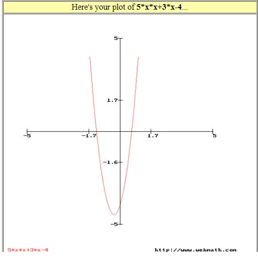
Lets take a super simple function ,an equation in one variable x , f(x) = 5x²-3x-4 which is representing  Loss Function. The plot of f(x) is a parabola as the function involves x² terms.  You can try plotting your algebraic expression at URL http://www.webmath.com/. The plot of our chosen algebraic expression is as shown in Fig 1.0 and we clearly see the function has a minimum value corresponding to some value of x( we will figure out this x value!).

 Our goal is to find a minimum of f(x) and calculus fundamentals indicate a minimum value of a function, we have the derivative,f'(x) =0. Here the derivative of f(x) is given by f'(x) = 10x+3 (derivative of 5x² is 2*5*x and derivative of 3x is 3 and derivative of constant is 0).

To reach a minimum point of our function, we start with an arbitrary point, say x₀=5. Then f'(x) at x=5 is 53. We introduce a new constant called eta (we will give it a name later!). So in our quest to find x corresponding to f(x) minimum , we traverse to x₁ = x₀-(eta*f'(x)) and keep moving in an iterative manner till the time we encounter f'(x) =0 .  Python is an excellent tool to automate such a boring task and we can use our coding skills here.

#import necessary libraries

import numpy as np

import pandas as pd

from scipy.misc import derivative

#define function which returns our f(x)

def f(x):
    return 5*x**2 + 3*x-4
#store successive derivative values in a list
derivative_list =[]
#inital value of x =4
i=4
#store all successive values of x in a list called x_list
x_list = [4]
# initialize eta
eta =0.001
Flag=True
#loop to find derivative and corresponding x
while Flag:
  #using scipy estimate derivate at a given x
  result = derivative(f,i, dx=1e-6)
  derivative_list.append(result)
  i=i-(eta*result)# get new value of x
  #if derivative is 0 ,time to break loop
  if result ==0:
    Flag=False
    break
  x_list.append(i)
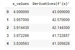
gradient_descent_df = pd.DataFrame({'x_values':x_list,'first_derivatives':derivative_list})
print(gradient_descent_df.head())

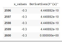
The output of the code is displayed in a dataframe for better appreciation. If we look at the first and last few rows it is seen that we have converged to f'(x) =0 after 2600 iterations at eta=0.001.

Analysis of Results

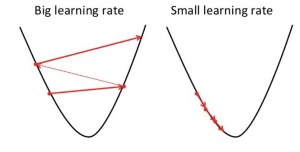
If we look at the output the f’(x) has finally converged to 0 with the corresponding value of x=-0.3.  In order to converge faster, we can also look at conditions where successive f’(x) is within an acceptable value, say 0.001. This will save us on computation and enable faster convergence. The eta value also plays a great part in our convergence. The eta value also called Learning Rate enables algorithm convergence and has to be chosen wisely. The Learning Rate is the rate at which we update the value of our parameter(x in our case). Initially, the steps are big but as we converge to our minimum, the steps are smaller. If we see our output dataframe first few rows and last few rows, the f'(x) values are high initially(hence we move with large step) and become small as we converge(approach minimum). A small Learning Rate will result in convergence taking longer iterations, but a higher learning rate may not converge and may end up in what we call oscillations. Please feel free to play around with the value of initial value and Learning Rate in the code and examine the outputs.

 

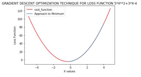
We can also plot the Gradient Descent algorithm for our simple Loss Function for visual appreciation. We see that blue curve shows our approach and is superimposed on the original Loss Function (marked in red).

# plot the loss function and gradient descent approach
def calculate_function(x):
  return 5*x**2+3*x-4
gradient_descent_df['Function_values'] = gradient_descent_df['x_values'].apply(calculate_function)
import matplotlib.pyplot as plt
plot_x = np.arange(-5,5,0.2)
plot_y = calculate_function(plot_x)
plt.plot(plot_x,plot_y,color='red',label='cost_function')
plt.plot(gradient_descent_df['x_values'],gradient_descent_df['Function_values'],label='Approach to Minimum')
plt.title('GRADIENT DESCENT OPTIMIZATION TECHNIQUE FOR LOSS FUNCTION 5*X**2+3*X-4')
plt.xlabel('Parameter')
plt.ylabel('Loss Function')
plt.legend()
plt.show()

Now solidifying our basic conceptual understanding, and extending the learning to the application of gradient Descent to ML problems, we will just introduce the concept rather than getting into details. We can represent a model output by a general function, Y = WX +B where Y is the output, X is the input and W and B represent weights and bias values. So the loss function will be a function involving W and B(our parameter in this case). As discussed earlier, our goal is to find out optimum values of W and B which will give us minimum loss function. So here we need to differentiate the loss function with respect to W and B. As two variables are involved we resort to partial differentiation (unlike earlier case had an f(x) with the only x), where if we have an f(x,y) in x and y then partial differentiation of f(x) with respect to x is obtained by keeping y as a constant and vice versa. In Gradient Descent, the iteration is similar to our earlier approach where W and B are initialized and the new values of W and B are found iteratively using Learning Rate and partial derivative till convergence. The Loss Function can get more complicated as a number of weights and bias increases for complex datasets, but the approach remains the same.

Conclusion

Gradient Descent algorithm is used in a large number of ML models and getting a grip on this concept is a good way of cementing our understanding of the Optimization Algorithm. It is suggested that with the conceptual understanding from this article, the reader can wade into the complexity of the application of GD on Linear Regression and Neural networks.

Subramanian Hariharan is a Marine Engineer with more than 30 Years of Experience and is passionate about leveraging Data for Business Solutions. 

Subramanian Hariharan 17 Jul 2021