Real or Not- Disaster Tweets Classification with RoBERTa

 This article was published as a part of the Data Science Blogathon.

Introduction

Today we live in a world of active social networking where every kind of information is shared among users worldwide. This is greatly facilitated by the ubiquitousness of smartphones and other handheld communication devices. Some popular sites are Facebook, Whatsapp, LinkedIn, etc.; however, Twitter is a viral microblogging site used worldwide for open information exchange.

On Twitter, various types of information are exchanged in the form of short messages that include information regarding any mishaps or accidents happening worldwide. It is seen that people prefer social networking sites like Twitter etc., more and more for such information exchange. In light of this, various disaster management agencies are also taking an active interest in retrieving information about any actual disaster happening at a certain location from such tweets. However, tweets being humongous in number, it is impossible to manually recognize each one of them as attributing to a real disaster or otherwise within a permissible time frame. Hence, the only way out is to leverage machine learning techniques for this task.

Machine Learning Problem

In the context of machine learning, the given task can be formulated as a Natural Language Processing problem where we need to classify a text (which is a tweet) as either referring to a real disaster or a fake one. Hence, essentially it is a two-class text classification task.

Following are some of the business constraints to the problem:

• There is no sub-second latency constraint. However, training or inference should not take too long to execute.
• Since disaster management agencies can use tweets or texts, prediction accuracy is paramount.
• Noise and Outliers are part of the dataset which need to be taken extreme care of to improve the model’s accuracy.

Dataset and the Data Structure

The dataset that will be used to model our task of predicting a tweet as either a real or fake disaster is taken from Kaggle. The dataset is part of an ongoing Kaggle competition in which anyone can participate. The dataset provided in Kaggle consists of two different sets, one is a train set that has manually labeled data for training any ML model, and the other is a test set that has no labeled data. Still, we need to make our prediction on this dataset. The Data structure of the given dataset is in a tabular form consisting of the following columns:

Hence the dataset essentially consists of five columns given as:

• The Id column gives a unique identifier to each data point
• The Keyword column gives the keyword in the text column with which the text is filtered
• The location column gives the place to which the tweet is referring
• The text column contains the description of the tweet
• The target contains the labels. Here the target is 1 for tweets referring to any real disaster and 0 for others

Performance Metrics

Before choosing our metric, let’s discuss some of the terms used in classification tasks:

• False Positives: These are those data points that are negative but are predicted positive
• False Negatives: These are those data points that are positive but are predicted negative
• True Positives: These are those data points that are correctly classified as positive
• True Negatives: These are those data points that are correctly classified as negative
• Precision: It is the ratio of the True Positives to the sum of True Positives and False Positives
• Recall: It is the ratio of the True Positives to the sum of True Positives and False Negatives
• F1-Score: It is the harmonic mean of Precision and Recall

Intuitively, Precision is how precise the model is in predicting positive points, and hence the more False Positives lesser would be the precision. Therefore, in cases where False Positive is costly, we need to take Precision as a metric for measuring the performance of a model.

On the other hand, Recall is the measure of how good our model is in correctly identifying the originally positive points. Hence the more False Negatives, the lesser would be the Recall. Therefore, in cases where False Negatives are costly, we need to take Recall as a metric for performance measurement.

F1-Score being the harmonic mean between Precision and Recall, it can simultaneously take both False Positives and False Negatives into account in the same metric.

In our case, the main aim is to predict if a tweets is referring to a real disaster and if it is, then mobilize the agencies to take action as fast as possible to reduce casualties. As we have to mobilize agencies, False Positives can be costly for them, and we have to save people’s lives in case of a real disaster; hence False Negatives can also be costly. As both False Positives and False Negatives are costly, we take the F1-score as our metric for comparing the performance of our models.

Importing important Libraries

Before starting our analysis, let’s import a bunch of libraries

import pandas as pd

import numpy as np

import re

import matplotlib.pyplot as plt

from wordcloud import WordCloud, STOPWORDS

import tensorflow as tf

Checking for Null-Values

We have already seen the data structure in the form of a table given earlier, so now let’s explore the data type in each of the columns and also the number of non-null values in them with the following API:

import pandas as pd
df = pd.read_csv('train.csv')
print(df.info())

From the above results, we can say that the columns id and target have integer type data, and the rest of them have string type data. Also, the columns, location, and keywords have many missing values, and the id column is just used as an identifier without having any ordinal significance. Since our focus is primarily on classifying the text data hence, we are removing these three columns and keeping only the text and target columns for further analysis.

Target Label Distribution

Through the following lines of codes, we are plotting the bar plot for the number of positive and negative data points

label_counts = df['target'].value_counts()
print(label_counts)
plt.figure(figsize=(3,3))
plt.bar(label_counts.index, label_counts,color ='maroon',
        width = 0.5)
plt.xlabel("Class Label")
plt.ylabel("Datapoint count")
plt.grid()
plt.show()

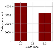
The number of data points for the negative class is 4342 and for the positive class is 3271. Therefore, the dataset is biased towards the negative class we need to account for later.

Text Cleaning

1. De-abbreviation

With this function named deabbreviate, we are expanding some of the abbreviated texts usually used in small messaging services.

def deabbreviate(text):
    text = text.upper()
    text = re.sub(r'bAFAIKb', ' As Far As I Know ',text)
    text = re.sub(r'bAFKb', ' From Keyboard ',text)
    text = re.sub(r'bASAPb', ' As Soon As Possible ',text)
    text = re.sub(r'bATKb', ' At The Keyboard ',text)
    text = re.sub(r'bA3b', ' Anytime, Anywhere, Anyplace ',text)
    text = re.sub(r'bBAKb', ' Back At Keyboard ',text)
    text = re.sub(r'bBBLb', ' Be Back Later ',text)
    text = re.sub(r'bBBSb', ' Be Back Soon ',text)
    text = re.sub(r'bBFNb', ' Bye For Now ',text)
    text = re.sub(r'bBRBb', ' Be Right Back ',text)
    text = re.sub(r'bBRTb', ' Be Right There ',text)
    text = re.sub(r'bBTWb', ' By The Way ',text)
    text = re.sub(r'bB4b', ' Before ',text)
    text = re.sub(r'bB4Nb', ' Bye For Now ',text)
    text = re.sub(r'bCUb', ' See You ',text)
    text = re.sub(r'bCUL8Rb', ' See You Later ',text)
    text = re.sub(r'bCYAb', ' See You ',text)
    text = re.sub(r'bFAQb', ' Frequently Asked Questions ',text)
    text = re.sub(r'bFYIb', ' For Your Information ',text)
    text = re.sub(r'bGNb', ' Good Night ',text)
    text = re.sub(r'bGR8b', ' Great ',text)
    text = re.sub(r'bICb', ' I See ',text)
    text = re.sub(r'bLOLb', ' Laughing Out Loud ',text)
    text = re.sub(r'bL8Rb', ' Later ',text)
    text = re.sub(r'bM8b', ' Mate ',text)
    text = re.sub(r'bTHXb', ' Thank You ',text)
    text = re.sub(r'bTTFNb', ' BYE ',text)
    text = re.sub(r'bTTFNb', ' BYE ',text)
    text = re.sub(r'bUb', ' You ',text)
    text = re.sub(r'bU2b', ' You TOO ',text)
    text = re.sub(r'bWTFb', ' What The Heck ',text)
    text = re.sub(r'bW8b', ' Wait ',text)
    text = re.sub(r'bFAVb', ' Favourite ',text)
    text = re.sub(r'bHWYb'," highway ",text)
    text = re.sub(r'bPPLb'," people ",text)
    text = re.sub(r'bGVb'," give ",text)
    text = re.sub(r'bWANNAb'," want to ",text)
    text = text.lower()
    return text

Twitter being a micro-blogging site, users usually tend to use a lot of abbreviated texts e.g., Lol, which essentially means Laughing Out Loud. Unless these texts are properly expanded, a machine cannot correctly get the context of a sentence completely. For example, if a sentence has the word laugh and another sentence has Lol, then a machine cannot comprehend that both refer to laughter. Hence, the de-abbreviation of texts becomes extremely important.

2. Filter Ascii

The above function filters out only the ASCII characters and removes any other non-ASCII or symbolic characters. 

def return_ascii(text):
    ret_str = ""
    for char in list(text):
        if char.isascii():
            ret_str += char
    return ret_str

We are filtering out those non-ASCII characters as they don’t add any value to the overall interpretation by any machine learning model.

3. General Preprocessing

Through the preprocess function, we are performing the data cleaning on the list of texts that are given to us in the form of tweets

punctuations = '!"#$%&()'*+,-./:;?@[]^_`{|}~'

def preprocess(text):

    #1.Removing AM and PM

    text = re.sub(r'b[AP]{1}Mb'," ",text)

    #2.Lowercasing 

    text = text.lower()

    #3.removing mentions

    text =re.sub(r'@[^ ]+',' ',text)

    #4.removing urls

    text = re.sub(r'https*://t.co/w+',' ',text)

    text = re.sub(r'https*://[^ ]+',' ',text)

    #5.De-abbreviating

    text = deabbreviate(text)

    #6.cleaning mscl

    text = re.sub(r"åê"," ",text)

    text = re.sub(r'&[^ ]+'," ",text)

    text = re.sub(r'b[a-z]+-[0-9]+b'," ",text)

    text = re.sub(r'bd+[a-z]+d+b'," ",text)

    text = re.sub(r'brtb'," ",text)

    text = re.sub(r'bfavb'," ",text)

    text = re.sub(r'b[h]{1}a[ha]+b',"haa",text)

    text = re.sub(r'b[a-z]+d+[a-z]+b'," ",text)

    text = re.sub(r'<[^]+>',' ',text)

    #7.removing months

    text = re.sub(r" jan | feb | mar | apr | may | jun | jul | aug | sep | oct | nov | dec ",' ',text)

    #8.decontracting

    text = re.sub(r"aren't",'are not',text)

    text = re.sub(r"won't",' will not ',text)

    text = re.sub(r"bi'mb",' I am ',text)

    text = re.sub(r"bi'db",' I would ',text)

    text = re.sub(r"bit'sb",' it is ',text)

    text = re.sub(r"bthat'sb",' that is ',text)

    text = re.sub(r"bcan'tb",' can not ',text)

    text = re.sub(r"bi'veb",' I have ',text)

    text = re.sub(r"bthere'sb",' there is ',text)

    text = re.sub(r"bdidn'tb",' did not ',text)

    text = re.sub(r"bcouldn'tb",' could not ',text)

    text = re.sub(r"bisn'tb",' is not ',text)

    text = re.sub(r"bwe'reb", ' we are ',text)

    text = re.sub(r"bthey'reb",' they are ',text)

    text = re.sub(r"bdon'tb",' do not ',text)

    text = re.sub(r"blet'sb",' let us ',text)

    text = re.sub(r"bli'lb",' little ',text)

    text = re.sub(r"bshe'sb",' she is ',text)

    text = re.sub(r"bhe'sb",' he is ',text)

    text = re.sub(r"bhow'reb",' How are ',text)

    text = re.sub(r"wasn't",' was not ',text)

    text = re.sub(r"bwhat'sb",' what is ',text)

    text = re.sub(r"bhe'llb",' he will ',text)

    text = re.sub(r"bi'llb",' i will ',text)

    text = re.sub(r"bshe'llb",' she will ',text)

    text = re.sub(r"byou'llb",' you will ',text)

    text = re.sub(r"byou'reb",' you are ',text)

    text = re.sub(r"bwe'veb",' we have ',text)

    text = re.sub(r"byou'veb",' you have ',text)

    text = re.sub(r"bthey'veb",' they have ',text)

    #9.removing expression

    text =re.sub(r'A[^ ]+:',' ',text)

    text =re.sub(r'A[^ ]+ [^ ]+:',' ',text)

    text =re.sub(r'A[^ ]+ [^ ]+ [^ ]+:',' ',text)

    #10.Removing the punctuations

    for p in punctuations:

        text = text.replace(p,"   ")

    #11.removing certain patters

    text = re.sub(r'lo+l',"laughing out loud",text)

    text = re.sub(r'coo+l',"cool",text)

    text = re.sub(r'go+a+l+','goal',text)

    text = re.sub(r'so+',"so",text)

    text = re.sub(r'bo+h+o*b','oh',text)

    #12.Removing the digits

    text = re.sub(r'd+'," ",text)

    #13.New line as space

    text = re.sub(r'n'," ",text)

    #14.Removing extra spaces

    text = re.sub(r'[ ]+'," ",text)

    #15.Stripping the end parts

    text = text.strip()

    #16.removing the accents

    text = return_ascii(text)

    #17.removing certain patterns after getting only the ascii characters

    text = re.sub(r"bcantb",' can not ',text)

    text = re.sub(r"bwontb",' will not ',text)

    text = re.sub(r"bimb",' I am ',text)

    text = re.sub(r"bdidntb",' did not ',text)

    text = re.sub(r"bcouldntb",' could not ',text)

    text = re.sub(r"bisntb",' is not ',text)

    text = re.sub(r"bdontb",' do not ',text)

    text = re.sub(r"blilb",' little ',text)

    text = re.sub(r"balilb",' a little ',text)

    text = re.sub(r"view and download video",' ',text)

    text = re.sub(r"bviaZ",' ',text)

    #18.Removing words with lengths less than 2

    text = [ele for ele in text.split(" ") if len(ele) > 1 ]

    text = " ".join(text)

    return text

Let’s look at the function serially:

1. We remove all the AM and PM expressions in the first step. We are removing it initially because they are associated with the time, which adds no value to a model, and secondly, AM may be misinterpreted as the verb am.
2. Here we are lower casing all the texts.
3. Tweets usually have mentions like @BBC or @Brial etc., which are non-essential for any model and hence are filtered out.
4. Sometimes there are URLs attached in the tweets referring to some sites. However, they don’t add any context to our interpretation and are removed.
5. We are de-abbreviating the text with the function mentioned above.
6. While going through the tweets, some unusual text sequences were found, e.g., texts within angled brackets or alpha-numeric texts, etc., which are usually noise sequences and are removed.
7. We are removing the names of different months in a year.
8. Next, we are de-contracting the text sequence so that it won’t and will not be interpreted similarly.
9. There are specific mentions at the beginning of sentences that end with a colon, e.g., “BBC NEWS: There is a large explosion in the town,” but here, BBC NEWS is adding no information and is rather redundant. Hence these types of expression are removed as well.
10. We are removing all the above-mentioned punctuation marks.
11. We are replacing some unusual expressions like loooool or gooaaalll etc., with the actual expression.
12. We are removing all the digits from the texts,
13. All the new-line characters are replaced with a space.
14. All the extra spaces are removed.
15. All the texts are stripped from left and right.
16. Non-ASCII characters are removed with the function mentioned above.
17. Some forms of contracted expression without apostrophes are de-contracted, e.g., didn’t or won’t, etc.
18. All single-character words are removed.

Data Preprocessing

After cleaning the text off the various noisy expression, we would be ready to double down on the data points in general. We would check various aspects of the dataset, e.g., what is the usual length of the tweets, are there any duplicates in the dataset, is there any ambiguous labeling done in the training dataset, what are the most frequently occurring words, and are they significant in classifying our intent?

1. Reading the dataset:

Now let’s again read the dataset from the disc, which is saved as train.csv, and apply the preprocessing that we have discussed so far

df = pd.read_csv("train.csv")
df = df.loc[:,['text','target']]
df['text'] = df['text'].apply(preprocess)

Here we are initially reading the training dataset contained in the file train.csv. Next, we are picking up only the text and target columns. Then the text data is preprocessed with the function mentioned above.

2. Removing any null values in the text column

After the text is cleaned, there might be instances that the whole text part is empty, and such data points cannot be fit into any model. Hence we need to drop such data points.

df.dropna(subset=['text'],inplace=True)

3. Removing all the duplicate text data and also data points with ambiguous labels

In the following lines of code, we are dropping all the same data points, and duplicating usually introduces bias in the model. Also, we are checking if there exists any exact data point which has been labeled as 1 as well as 0 and dropping them outright as these data points are ambiguous and introduce noise to the model.

df_dup = df[df['text'].duplicated()]
text_arr = np.unique(df_dup['text'].values)
df_dup = df[df['text'].isin(text_arr)].sort_values(by=['text'])
df_dup = df_dup[~df_dup.duplicated()].sort_values(by=['text'])
df_dup_contradiction = df_dup[df_dup['text'].duplicated()]
df_dup_contradiction.to_csv("ambiguous_datapoints_bert.csv")
df_dedup = df.drop_duplicates(subset=['text'])
df_dedup = df_dedup[~df_dedup['text'].isin(df_dup_contradiction['text'].values)]

4. Getting the information about the new data set

Now let’s take a quick look at the summary of the dataset after cleaning and pre-processing

df_dedup.info()

Int64Index: 6658 entries, 0 to 7606
Data columns (total 2 columns):
 #   Column  Non-Null Count  Dtype 
---  ------  --------------  ----- 
 0   text    6658 non-null   object
 1   target  6658 non-null   int64 
dtypes: int64(1), object(1)
memory usage: 156.0+ KB

The data frame df_dedup is our final dataset cleaned of all the noisy texts. Also, all the duplicate entries in the dataset are removed, and those data points are removed if any duplicate datapoint has ambiguous labels.

5. Plotting the percentile plot of review length

After all the cleaning and preprocessing, let’s take a look at the distribution of the number of words in the texts and get a sense of the maximum and minimum tweet length

review_len = np.array([len(x.split()) for x in df_dedup['text'].values])
review_len = np.sort(review_len)
review_len_percnt = np.percentile(review_len,range(100))
fig = plt.figure(figsize=(7,7))
ax = fig.add_subplot(111)
ax.plot(range(100),review_len_percnt)
ax.set_xlabel("Percentile")
ax.set_ylabel("Review Length")
plt.grid()
plt.show()

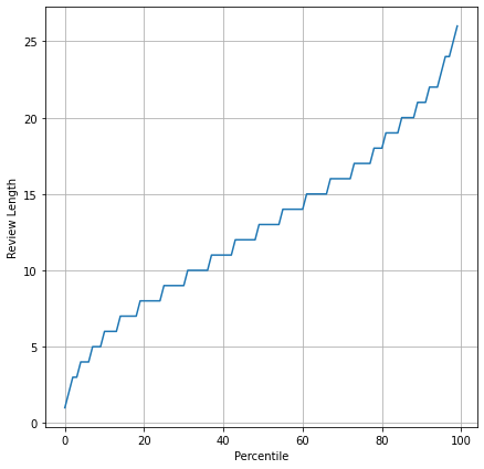
From the above percentile distribution, we can see that the max length of the tweet is just more than 25, which is well within permissible limits for any machine learning model.

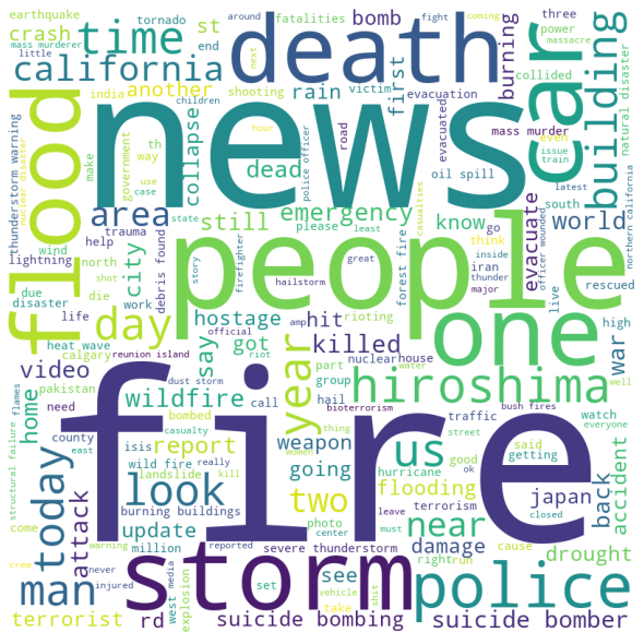
6. WordCloud for positive reviews

Word Cloud gives us an intuition regarding the frequency of occurrence of a word in a given corpus. The higher the frequency, the bigger the font size. So from the word cloud, we can get an idea about the words dominating in a particular class of tweets. Here we draw the word cloud for the positively labeled text data points.

positive_sentences = ""
for sentence in df_dedup[df_dedup['target'] == 1]['text'].tolist():
    positive_sentences = positive_sentences + " "+sentence
stopwords = set(STOPWORDS)
wordcloud = WordCloud(width = 800, height = 800,
                background_color ='white',
                stopwords = stopwords,
                min_font_size = 10).generate(positive_sentences)
# plot the WordCloud image                      
plt.figure(figsize = (8, 8), facecolor = None)
plt.imshow(wordcloud)
plt.axis("off")
plt.tight_layout(pad = 0)
plt.show()

7. WordCloud for negative reviews

Here we are drawing the word cloud for the negatively labeled text data points

negative_sentences = ""
for sentence in df_dedup[df_dedup['target'] == 0]['text'].tolist():
    negative_sentences = negative_sentences + " "+sentence
stopwords = set(STOPWORDS)
wordcloud = WordCloud(width = 800, height = 800,
                background_color ='white',
                stopwords = stopwords,
                min_font_size = 10).generate(negative_sentences)
# plot the WordCloud image                      
plt.figure(figsize = (8, 8), facecolor = None)
plt.imshow(wordcloud)
plt.axis("off")
plt.tight_layout(pad = 0)
plt.show()

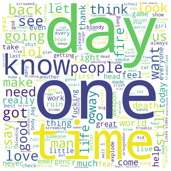
As we can see, words like fire, storm, death, flood, etc. dominate the real disaster tweets and words like day, one, time, etc. dominate the fake ones.

Modeling

1. Train Test Split

Through these following lines of code, we are splitting the given dataset into training and test dataset.

from transformers import AutoTokenizer, TFAutoModelForSequenceClassification

from sklearn.model_selection import train_test_split

X_train, X_test, y_train, y_test = train_test_split(df_dedup['text'],df_dedup['target'], stratify=df_dedup['target'],random_state=35,test_size=0.1)

We are importing the train_test_split API of scikit-learn for splitting our train dataset. We are here keeping 90% of the data for training the RoBERTa model and 10% as validation data. As we have already seen that the dataset has a class imbalance, and hence we are using stratified sampling for the split.

2. Tokenization

Here the cleaned text is converted into tokens for feeding into the model

tokenizer = AutoTokenizer.from_pretrained("roberta-base") #Tokenizer
train_inputs = tokenizer(X_train.tolist(), padding=True, truncation=True, return_tensors='tf') #Tokenized text
train_labels = y_train
test_inputs = tokenizer(X_test.tolist(), padding=True, truncation=True, return_tensors='tf') #Tokenized text
test_labels = y_test

As we all know, machines can’t interpret English texts; somehow, we need to convert the texts to some form of numerical representation. The above step is essentially a way to convert text to numbers. Here we use a pre-trained tokenizer from a popular NLP library called Hugging-Face with the check-point name roberta-base.

Tokenization is slicing the text into various pieces and assigning each slice a token number. Say we have a text, “The pizza is very delicious,” then the tokenizer would slice it into various sub-texts and map each to a number. Various forms of tokenization exist character-level tokenization, word-level tokenization, and sub-word tokenization. The tokenization that the RoBERTa model uses is a type of sub-word tokenization called Byte-Level Byte Pair Encoding.

The tokenizer takes the following arguments:

1. A list of texts to tokenize
2. padding argument, which is a boolean value indicating should the shorter texts in the corpus be padded with dummy values
3. truncation is also a boolean value indicating should the longer texts be truncated.
4. return_tensor gives the type of tensor to return since we are working in a tensorflow environment, so we give the type as ‘tf’, which stands for TensorFlow.

The returned tensor has two essential lists: First, the tokens, and second, the attention mask, which indicates which are the real tokens and which are padded tokens.

3. Training

The LossOnHistoryRobert is a custom callback class used for printing the confusion matrix and F1 score.

class LossOnHistoryRobert(tf.keras.callbacks.Callback):

    def __init__(self,x_val,y_val):

        self.x_val = x_val

        self.y_val = y_val

    def on_train_begin(self, logs={}):

        self.history={'loss': [],'accuracy': [],'val_loss': [],'val_accuracy': [],'val_f1': []}

    def on_epoch_end(self, epoch, logs={}):  

        true_positives=0

        self.history['loss'].append(logs.get('loss'))

        self.history['accuracy'].append(logs.get('accuracy'))

        if logs.get('val_loss', -1) != -1:

            self.history['val_loss'].append(logs.get('val_loss'))

        if logs.get('val_accuracy', -1) != -1:

            self.history['val_accuracy'].append(logs.get('val_accuracy'))

        #y_pred gives us the probability value 

        y_pred= self.model.predict(self.x_val)

        y_pred = np.argmax(np.array(y_pred.logits),axis=1)

        #The micro_f1 score

        f1 = f1_score(self.y_val.values, y_pred)

	#confusion_matrix

        print(confusion_matrix(self.y_val.values, y_pred))

        self.history['val_f1'].append(f1)

        print('F1_Score: ',f1)

model = TFAutoModelForSequenceClassification.from_pretrained("roberta-base", num_labels=2)

model.compile(

        optimizer=tf.keras.optimizers.Adam(learning_rate=0.00001, clipnorm=1.),

        loss=tf.keras.losses.SparseCategoricalCrossentropy(from_logits=True),

        metrics=[tf.metrics.SparseCategoricalAccuracy()],

        )

In the above lines of code, we have initially defined a custom callback class that shows the Confusion matrix and the F1-Score at the end of each epoch. Next, we initialize a pre-trained roberta-base model from the Hugging Face library with the number of class labels as 2, as we are doing a two-class classification. Then we have defined the loss function as SparseCategoricalCrossentropy with from logits as True as the model output is not normalized. Then we use an Adam optimizer with a learning rate of 0.00001 and defined the metric as SparseCategoricalAccuracy.

history_own=LossOnHistoryRobert(dict(test_inputs),test_labels) 
history=model.fit(dict(train_inputs),train_labels, validation_data=[dict(test_inputs),test_labels], batch_size=32,epochs=1, verbose=1, callbacks=history_own)

Here the pre-trained model is fitted with the train and validation data. We have also passed the custom callback object to keep track of the F1-Score and kept the batch size as 32. The batch size may vary depending on the hardware configuration. After running the model through 10 epochs following was the result.

[[388   6]
 [ 15 257]]
F1_Score:  0.9607476635514018
188/188 [==============================] - 68s 266ms/step - loss: 0.1567 - sparse_categorical_accuracy: 0.9438 - val_loss: 0.0905 - val_sparse_categorical_accuracy: 0.9685

As we can see, we could get a very nice F1_score of around 0.96. However, we could also tweak with other hyper-parameters to make the score even better. But I am leaving it as an exercise for the readers to try and comment on.

Inference

This section will see how to make inferences from a fully trained model given a set of tweets. For that, we are defining a function called final which takes a list of tweets as an argument. The tweets are initially cleaned with the help of the preprocess function, which we discussed earlier. After getting the cleaned-up text, we tokenize them with the help of the pre-trained BPE tokenizer, and finally, the tokenizer output is fed to the fine-tuned RoBERTa model, which returns a set of logits as output. The logits are obtained as a list of lists, and the inner list has only two values such that if the value at the second position is more than that at the first one, then the label is predicted as 1 otherwise, 0. And further, this logic is processed to determine if the tweet is referring to a disaster or not to any disaster.

def final(*args):

    output_lst = []

    for x in args:

        x = preprocess(x)

        x = tokenizer(x,return_tensors='tf')

        x = model(x).logits

        if x.numpy()[0][0] > x.numpy()[0][1]:

            output_lst.append("Not referring to any disaster.")

        else:

        output_lst.append("Referring to a disaster.")

return output_lst

final("There is a #fire& in the building",
     "The sun is shining bright today @safolla http://www.vtv.com",
     "#BBCworld Hey #God save us....There is an earthquake")
['Referring to a disaster.',
 'Not referring to any disaster.',
 'Referring to a disaster.']

Conclusion

In this article, we have seen the entire pipeline for a binary text classification problem statement, particularly for recognizing whether a tweet is a real disaster or a fake one.

Following are the important points from our discussion on tweet classification:

• Cleaning the text off the various noisy expressions and characters
• Dropping the data points having duplicate entries as duplication introduces bias in the model
• Dropping those data points having ambiguous labels to the text data
• Tokenizing the text data with a sub-word tokenizer known as Byte-Level Byte Pair Encoding
• Modeling the tokenized data with the state-of-the-art RoBERTa model
• Taking inference from the trained model with some query points

Thanks for reading this article, and let me know through comments if you found the article useful.

The media shown in this article is not owned by Analytics Vidhya and is used at the Author’s discretion.

Abhijit