A Beginner’s Guide to Focal Loss in Object Detection!

Introduction

Object detection is one of the most widely studied topics in the computer vision community. It’s has been breaking into various industries with use cases from image security, surveillance, automated vehicle systems to machine inspection.

Currently, deep learning-based object detection can be majorly classified into two groups:-

1. Two-stage detectors, such as Region-based CNN (R-CNN) and its successors.
2. and, One-stage detectors, such as the YOLO family of detectors and SSD

One-stage detectors that are applied over a regular, dense sampling of anchor boxes (possible object locations) have the potential to be faster and simpler but have trailed the accuracy of two-stage detectors because of extreme class imbalance encountered during training.

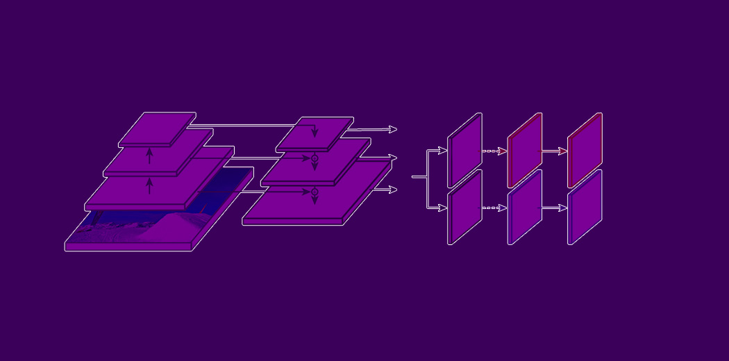
FAIR has released a paper in 2018, in which they introduced the concept of Focal loss to handle this class imbalance problem with their one stage detector called RetinaNet.

Before we deep dive into the nitty-gritty of Focal loss, let’s First, understand what is this class imbalance problem and the possible problems caused by it.

Table of Contents

1. Why Focal Loss Needed
2. What is Focal Loss
3. Cross-Entropy Loss
   1. Problem with Cross-Entropy
   2. Examples
4. Balanced Cross-Entropy
   1. Problem with Balanced Cross-Entropy
   2. Examples
5. Focal loss explanation
   1. Examples
6. Cross-Entropy vs Focal Loss
   1. Easily correctly classified records
   2. Misclassified records
   3. Very easily classified records
7. Final Thoughts

Why Focal Loss Needed?

Both classic one stage detection methods, like boosted detectors, DPM & more recent methods like SSD evaluate almost 10⁴ to 10⁵ candidate locations per image but only a few locations contain objects (i.e. Foreground) and rest are just background objects. This leads to the class imbalance problem.

This imbalance causes two problems –

1. Training is inefficient as most locations are easy negatives (meaning that they can be easily classified by the detector as background) that contribute no useful learning.
2. Since easy negatives (detections with high probabilities) account for a large portion of inputs. Although they result in small loss values individually but collectively, they can overwhelm the loss & computed gradients and can lead to degenerated models.

What is Focal Loss?

In simple words, Focal Loss (FL) is an improved version of Cross-Entropy Loss (CE)  that tries to handle the class imbalance problem by assigning more weights to hard or easily misclassified examples  (i.e. background with noisy texture or partial object or the object of our interest ) and to down-weight easy examples (i.e. Background objects).

So Focal Loss reduces the loss contribution from easy examples and increases the importance of correcting misclassified examples.)

So, let’s first understand what Cross-Entropy loss for binary classification.

Cross-Entropy Loss

The idea behind Cross-Entropy loss is to penalize the wrong predictions more than to reward the right predictions.

Cross entropy loss for binary classification is written as follows-

Where –

Y_act = Actual Value of Y

Y_pred =  Predicted Value of Y

For Notational convenience, let’s write Y_pred  as p & Y_act as Y.

Y ∈ {0,1}, It’s the ground truth class

p ∈ [0,1], is the model’s estimated probability for the class with Y=1.

For notational convenience, we can rewrite the above equation as –

p_t = {-ln(p)         , when Y=1 -ln(1-p)    ,when Y=}

CE (p, y) = CE (p_t)=-ln⁡(p_t)

Problem with Cross-Entropy

As you can see, the blue line in the below diagram, when p is very close to 0 (when Y =0) or 1, easily classified examples with large p_t > 0.5 can incur a loss with non-trivial magnitude.

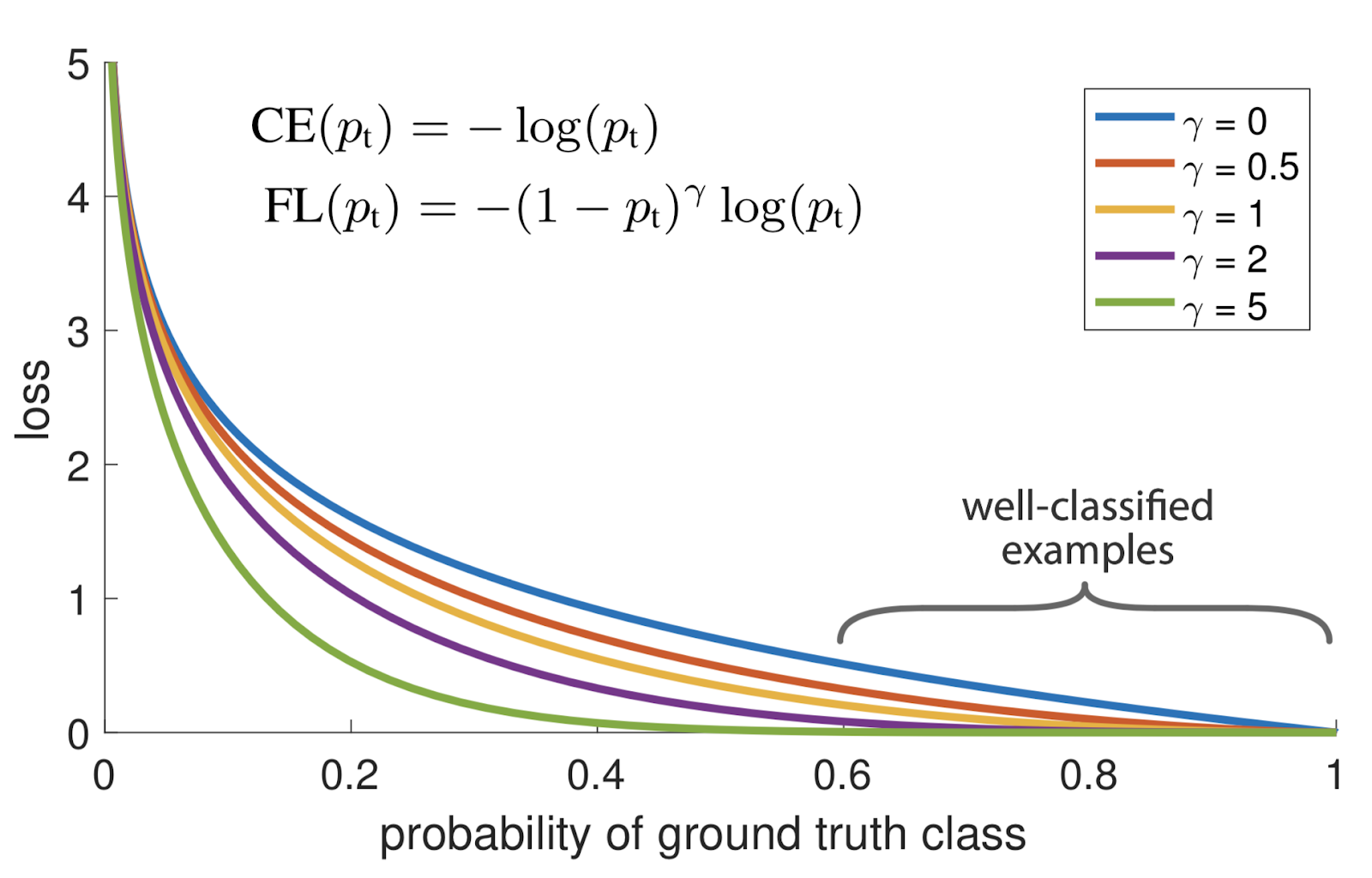
Fig: – The focal loss down weights easy examples with a factor of  (1-  p_t)^γ

Let’s understand it using an example below-

Examples: –

Let’s say, Foreground (Let’s call it class 1) is correctly classified with p=0.95 –
CE(FG) = -ln (0.95) =0.05

And background (Let’s call it class 0) is correctly classified with p=0.05 –
CE(BG)=-ln (1- 0.05) =0.05

The problem is, with the class imbalanced dataset, when these small losses are sum over the entire images can overwhelm the overall loss (total loss).  And thus, it leads to degenerated models.

Balanced Cross-Entropy Loss

A common approach to addressing such a class imbalance problem is to introduce a weighting factor ∝∈[0,1] for class 1 & 1- for class -1.

For notational convenience, we can define ∝_t in loss function as follows-

CE (p_t )= -∝_tln ln( p_t )

As you can see, this is just an extension to Cross-Entropy.

Problem with Balanced Cross-Entropy: –

As our experiments will show, the large class imbalance encountered during the training of dense detectors overwhelms the cross-entropy loss.

Easily classified negatives comprise the majority of the loss and dominate the gradient. While balances the importance of positive/negative examples, it does not differentiate between easy/hard examples.

Let’s understand this with an example-

Examples: –

Let’s say, Foreground (Let’s call it class 1) is correctly classified with p=0.95 –
CE(FG) = -0.25*ln (0.95) =0.0128

And background (Let’s call it class 0) correctly classified with p=0.05 –
CE(BG)=-(1-0.25) * ln (1- 0.05) =0.038

While it does a good job differentiating positive & negative classes correctly but still does not differentiate between easy/hard examples.

And that’s where Focal loss (extension to cross-entropy) comes to rescue.

Focal loss explanation

Focal loss is just an extension of the cross-entropy loss function that would down-weight easy examples and focus training on hard negatives.

So to achieve this,  researchers have proposed:
(1-  p_t)^γ  to the cross-entropy loss, with a tunable focusing parameter γ≥0.

RetinaNet object detection method uses an α-balanced variant of the focal loss, where α=0.25, γ=2 works the best.

So focal loss can be defined as –

FL (p_t) = -α_t(1-  p_t)^γ log  log(p_t).

The focal loss is visualized for several values of γ∈[0,5], refer Figure 1.

We shall note the following properties of the focal loss-

1. When an example is misclassified and p_t is small, the modulating factor is near 1 and the loss is unaffected.
2. As
   p_t→  1, the factor goes to 0 and the loss for well-classified examples is down weighed.
3. The focusing parameter
   γ smoothly adjusts the rate at which easy examples are down-weighted.

As is increased, the effect of modulating factor is likewise increased. (After a lot of experiments and trials, researchers have found γ = 2 to work best)

Note:- when γ =0, FL is equivalent to CE. Shown blue curve in Fig

Intuitively, the modulating factor reduces the loss contribution from easy examples and extends the range in which an example receives the low loss.

Let’s understand the above properties of focal loss using an example-

Examples: –

• When record (either foreground or background) is correctly classified-

1. The foreground is correctly classified with predicted probability p=0.99 and background are correctly classified with predicted probability p=0.01.
   p_t = {0.99, when Y_act=1 1-0.01 ,when Y_act = 0}Modulating factor (FG)= (1-0.99)² = 0.0001
   Modulating factor (BG)= (1-(1-0.01))² = 0.0001As you can see, the modulating factor is close to 0, in turn, the loss would be down-weighted.
2. The foreground is misclassified with predicted probability p=0.01 for background object misclassified with predicted probability p=0.99.
   p_t = {0.01, when Y_act=1 1-0.99 ,when Y_act = 0}Modulating factor (FG)= (1-0.01)² =0.9801
   Modulating factor (BG)= (1-(1-0.99))² =0.9801As you can see, the modulating factor is close to 1, in turn, the loss is unaffected.

Now let’s compare Cross-Entropy and Focal loss using a few examples and see the impact of focal loss in the training process.

Cross-Entropy vs Focal Loss

Let’s see the comparison by considering a few scenarios below-

• Easily correctly classified recordsLet’s say Foreground is correctly classified with predicted probability p=0.95 and background is correctly classified with predicted probability p=0.05.
  p_t = {0.95, when Y_act=1 1-0.05 ,when Y_act = 0}CE(FG)= -ln (0.95)    = 0.0512932943875505
  CE(BG)= -ln (1-0.05) = 0.051293294387550
  Let’s consider the same scenario Focal loss with ∝=0.25 & γ =2.
  
  FL(FG)= -0.25 * (1-0.95)² *ln (0.95) = 3.2058308992219E-5
  FL(BG)=-0.75 * (1-(1-0.05))² *ln (1-0.05) =9.61E-5

• Misclassified records
  Let’s say the foreground is classified with predicted probability p=0.05 for background object misclassified with predicted probability p=0.95.
  p_t = {0.95, when Y_act=1 1-0.05 ,when Y_act = 0}
  
  CE(FG)= -ln (0.05)    = 2.995732273553991
  CE(BG)= -ln (1-0.95) = 2.995732273553992Let’s consider the same scenario Focal loss with ∝=0.25 & γ =2.
  
  FL(FG)= -0.25 * (1-0.05)² *ln (0.05) = 0.675912094220619
  FL(BG)= -0.75 * (1-(1-0.95))² *ln (1-0.95) =2.027736282661858  

• Very easily classified records
  Let’s say the foreground is classified with predicted probability p=0.99 for background object misclassified with predicted probability p=0.01.
  p_t = {0.99, when Y_act=1 1-0.01 ,when Y_act = 0}CE(FG)= -ln (0.99)    = 0.0100503358535014
  CE(BG)= -ln (1-0.01) = 0.0100503358535014Let’s consider the same scenario Focal loss with ∝=0.25 & γ=2.
  
  FL(FG)= -0.25 * (1-0.01)² *ln (0.99) = 2.51*10^-7
  FL(BG)= -0.75 * (1-(1-0.01))² *ln (1-0.01) =7.5377518901261E-7

Final Thoughts

scenario-1: 0.05129/3.2058*10^-7 = 1600 times smaller number
scenario-2: 2.3/0.667 = 4.5 times smaller number
scenario-3: 0.01/0.00000025 = 40,000 times smaller number.

These three cases clearly explain how Focal loss adds down weights the well-classified records and on the other hand, assigns large weight to misclassified or hard classified records.

After a lot of trials and experiments, researchers have found ∝=0.25 & γ=2 to work best.

End Points

We went through the complete journey of evolution of cross-entropy loss to a focal loss in object detection.  I’ve tried my bit to explain the focal loss in object detection as simple as possible. Please feel free to comment on your queries. I’ll be more than happy to answer them.

If you enjoyed this article, leave a few claps, it will encourage me to explore more machine learning techniques & pen them down 🙂

Happy learning. Cheers!!

References: –

https://arxiv.org/ftp/arxiv/papers/2006/2006.01413.pdf
https://medium.com/@14prakash/the-intuition-behind-retinanet-eb636755607d
https://developers.arcgis.com/python/guide/how-retinanet-works/

About the Author

Praveen Kumar Anwla

I’ve been working as a Data Scientist with product-based and Big 4 Audit firms for almost 5 years now. I have been working on various NLP, Machine learning & cutting edge deep learning frameworks to solve business problems. Please feel free to check out my personal blog, where I cover topics from Machine learning – AI, Chatbots to Visualization tools ( Tableau, QlikView, etc.) & various cloud platforms like Azure, IBM & AWS cloud.