This article was published as a part of the Data Science Blogathon.
Introduction on Walmart Stock Price
In this article, we will be analyzing the famous Walmart Stock Price dataset using PySpark’s data preprocessing techniques here we will start everything from the very beginning and at the end of this article, one will experience the feel of the consulting project as we will be answering some of the professional financial questions to ourselves based on our analysis.
Mandatory Steps to follow:
- Starting the spark session: In this segment, we will set up the spark session to use it with the python’s distribution of Spark i.e. PySpark.
- Reading the dataset: In this section, we will be reading the Walmart stock price data that I have first downloaded from Kaggle, and then extracted the stock data from 2012-to 2017 and we will be analyzing the data for these years only in this particular blog.
Let’s get started and analyze the Walmart stocks using PySpark
Setting up a simple Spark Session
This is one of the mandatory things to do before getting started with PySpark i.e. to set up an environment for Spark to use the python’s PySpark library and use all of its resources in that session.
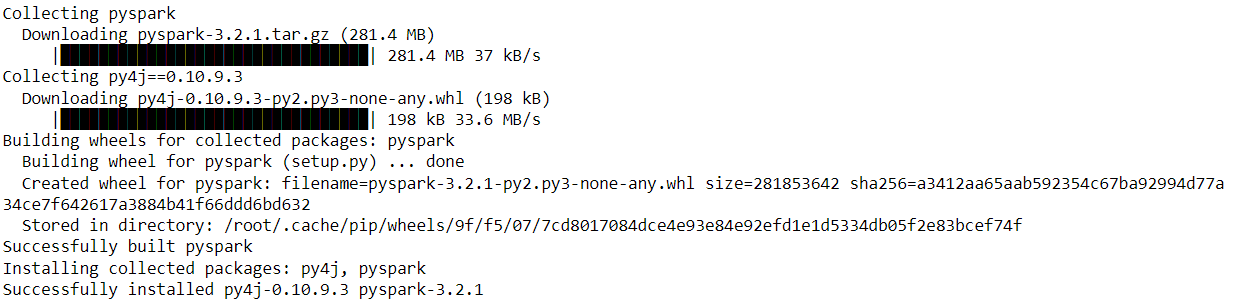
Note: Before importing kinds of stuff don’t forget to install the PySpark library, Command to install the library is: pip install pyspark.
!pip install pyspark
Output:
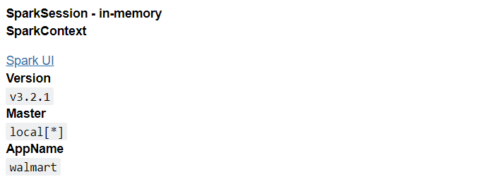
from pyspark.sql import SparkSession

spark_walmart = SparkSession.builder.appName("Walmart_Stock_Price").getOrCreate()
spark_walmart
Output:
Code Breakdown
Here we will break down the above code and understand each element required for creating and starting the Spark environment.
- Firstly we have imported the SparkSession object from the pyspark.sql library and this object will hold all the curated functions that are required.
- Then using the SparkSession object we are calling the builder function which will build the session and give the specific name to the session using AppName at the end we will create the environment using the getOrCreate() function.
- At the last, we will be looking at Spark UI which curates all the necessary information about Spark’s environment like its version, Branch (Master), and the AppName.
Reading the Walmart Stock Price Data
In this section, we will be reading Walmart’s stock price data using PySpark and storing it in the variable to use for further analysis. As we know that in pandas we used CSV() function similarly we use the read.csv() function in PySpark. Let’s further discuss the same.
df = spark_walmart.read.csv('walmart_stock.csv',header=True,inferSchema=True)
df.show()
Output:
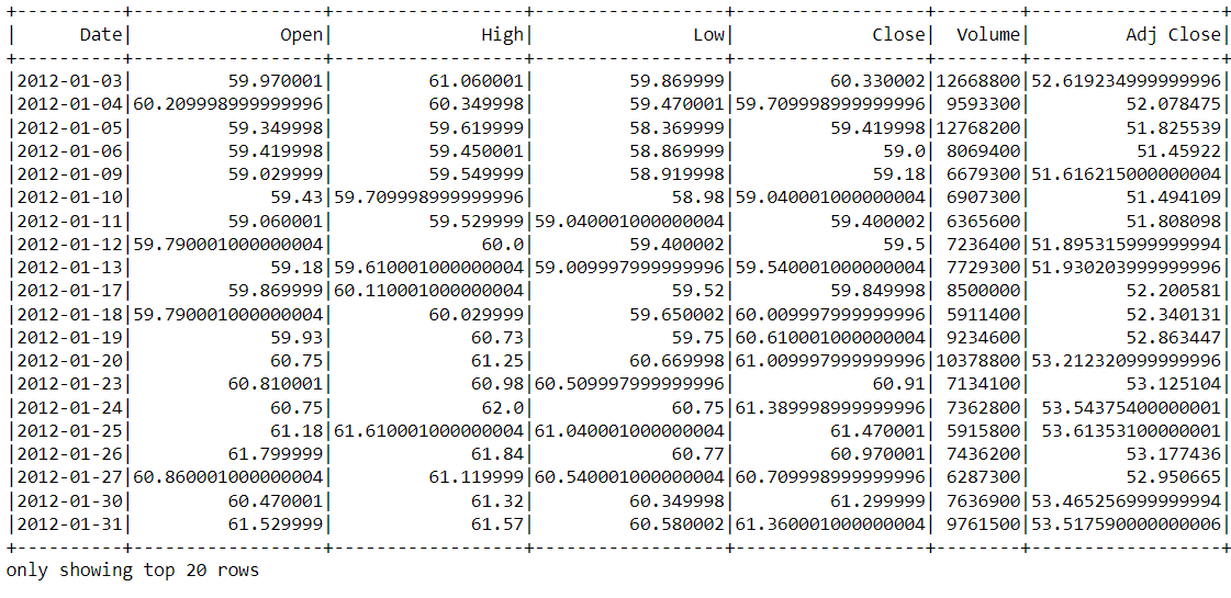
Inference: Here we can see that show() function has returned the top 20 rows of the dataset. Note that we have kept the header type as True so that spark will treat the first row as header and inferSchema is also set to True so that it returns the values with the real data type.
Understanding the Dataset
In this section we will be using the relevant functions of PySpark to analyze the dataset from analyzing here I mean that we will see what our dataset looks like, what is the structure of the same and what formatting needs to be done as a cleaning part.
Here are the following things that we will be covering here:
- Looking at the name of the columns that Walmart data holds.
- Understanding the Schema of the dataset.
- Looping through the specific number of rows in the data.
- Understanding the statistical information that our data signifies.
Let’s have a look at the column’s names.
df.columns
Output:
['Date', 'Open', 'High', 'Low', 'Close', 'Volume', 'Adj Close']
Inference: From the above output we can see that it returned the list of values where ‘values’ denotes the name of the columns which are present and for that we used the columns object.
Now we will see what the schema of the dataset looks like!
df.printSchema()
Output:
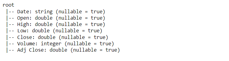
Inference: Here, using the print schema() function, we are actually looking at the data type of each column of the dataset and here we can note one thing as well: “nullable = True” signifies that the column can hold the NULL values.
Looping through the data and fetching the top 5 rows.
for row in df.head(5):
    print(row)
    print('n')
Output:
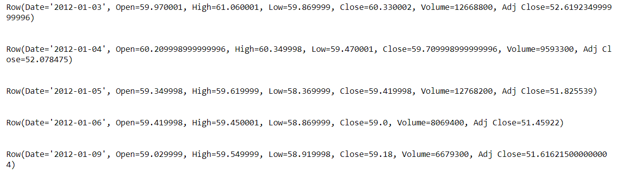
Inference: In the above output we can see that it returned the “ROW” object and in this row object it holds the real top 5 data ( because we iterated through top 5 data using the head() function ) and this is one of the ways where we can extract the one or multiple tuples of record separately.
Note: This is a completely optional thing to involve in this analysis as we will be using this concept if we want to hold each row in a different variable to play with each data point.
Using describe() function to see the statistical information of the dataset.
Formatting the Dataset
In this section we will format our dataset to make it clearer and more precise so that we will have clean data which will be easier to analyze than the current state of the data as the inferences which we will draw now will not give a clearer picture of the results.
Hence here we will first format some of the columns to their nearest integer value and along with that add one column too for avoiding further calculations
So let’s format our dataset and perform each step one by one:
Before moving further and changing the formatting of the data points let us first see on what columns we have to apply those changes and for that we will use the combination of printSchema and describe the function.
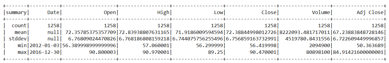
df.describe().printSchema()
Output
Inference: In the above output we can see the data type of each method that was returned by describing the function and from the output, we can see that all the columns hold the string values which is not good if we want to format them and further analyze them
Hence now it’s our task to first change the data type of these columns (specifically for mean and standard deviation) and later format it for better understanding.
As discussed earlier, now as we know what to do its time to know how to do and to answer this question we will be using the format_number function from the “functions” package and this will help us to,
- Firstly change the data type of the column to the relevant type
- Secondly, it will also convert the values to the nearest integer.
from pyspark.sql.functions import format_number

result = df.describe()
result.select(result['summary'],
              format_number(result['Open'].cast('float'),2).alias('Open'),
              format_number(result['High'].cast('float'),2).alias('High'),
              format_number(result['Low'].cast('float'),2).alias('Low'),
              format_number(result['Close'].cast('float'),2).alias('Close'),
              result['Volume'].cast('int').alias('Volume')
             ).show()
Output:
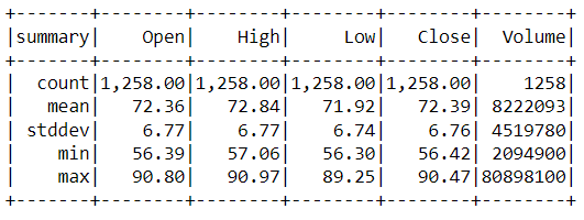
Code Breakdown
- In this first step of formatting the data, we have imported the format_number class from the functions package of pyspark.
- Then, as we already knew that we have to change the data of mean and standard deviation so based on that described method has been used and stored in the separate variable.
- Then comes the main thing where firstly select statement is used (equally to SQL’s select statement) and here,
- the cast function is used to change the data type (typecasting) and set the decimal values after a point.
- alias function is used to change the column name (not permanently just for first-time view)
Now let’s create an altogether new DataFrame which will have one column named HV ratio which will stimulate the ratio of High Price and Total Volume of stock which were traded for a day.
df2 = df.withColumn("HV Ratio",df["High"]/df["Volume"])
df2.select('HV Ratio').show()
Output:
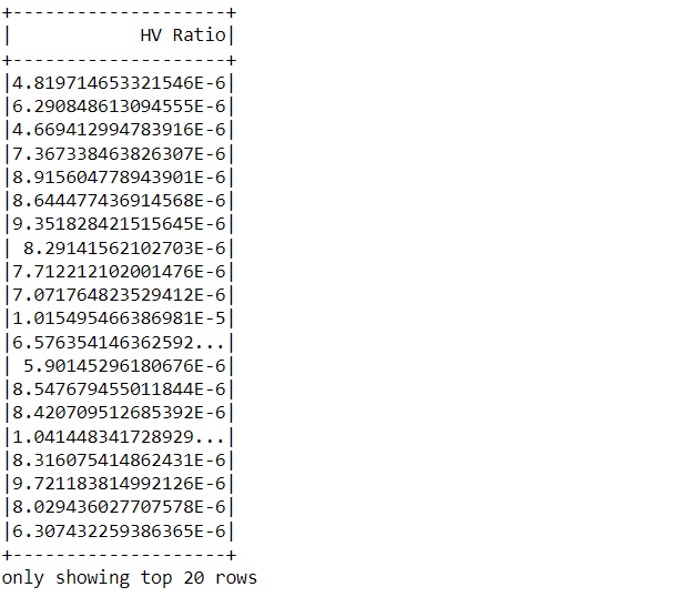
Inference
Here in the output, one can see that this new DataFrame holds the ratio of discussed fields, we introduced the column in this DataFrame with the help of the “with column()” function and then simply performed the ratio operation and showed it with a combination of select and show statement.
Enough of preparing the dataset! We are supposed to analyze Walmart’s Stock Price and now it’s time for it!
Questions to Analyze Using PySpark
In this section, we will give answers to some questions proposed to us by a firm to give us a feel of the data science consulting projects here we will draw the insights using the PySpark’s data preprocessing technique
- On what day stock price was the highest?
- What is the average Closing price?
- What is the maximum and minimum volume of stock traded
- For how many days the closing value was less than 60 dollars?
- What could be the maximum high value for each year?
- On what day stock price was the highest?
df.orderBy(df["High"].desc()).head(1)[0][0]
Output:
'2015-01-13'
Inference: In the above output we can see that we got the date on which stock price was highest by using the orderly function and selecting it in descending order then we have simply used the head function with a little bit of indexing to fetch the data object from the data
- What is the average Closing price?
from pyspark.sql.functions import mean
df.select(mean("Close")).show()
Output:
+-----------------+
|       avg(Close)|
+-----------------+
|72.38844998012726|
+-----------------+
Inference: From the above output we can say that the average closing price is 72.38844998012726 and we have fetched this value by using the select statement and then the mean function to show the mean closing stock price
Note: Here we could have also used the describe method but I wanted you to know the operations that are possible with PySpark
- What is the maximum and minimum volume of stock traded?
from pyspark.sql.functions import max,min

df.select(max("Volume"),min("Volume")).show()
Output:
+-----------+-----------+
|max(Volume)|min(Volume)|
+-----------+-----------+
|   80898100|    2094900|
+-----------+-----------+
Inference: To get the maximum and minimum volume of the stocks we first imported the “max” and “min” functions using the “functions” package and then it’s like walking on the cake, we have simply used these functions to get the desired results using select statements. Here also we can use the describe function.
- For how many days the closing value was less than 60 dollars?
df.filter(df['Close'] < 60).count()

from pyspark.sql.functions import count
result = df.filter(df['Close'] < 60)
result.select(count('Close')).show()
Output:
+------------+
|count(Close)|
+------------+
|          81|
+------------+
Inference: Now to get the total number of days to get the closing value which is less than 60 dollars we have to follow two steps to get the desired results:
- Using the filter operations we are filtering the closing value less than 60 so we could get the required data only and then with the count function counting the total number of filtered records.
- Then we are simply using the select statement and putting everything in this select statement
- What could be the maximum high value for each year?
from pyspark.sql.functions import year
yeardf = df.withColumn("Year",year(df["Date"]))

max_df = yeardf.groupBy('Year').max()

max_df.select('Year','max(High)').show()
Output:
+----+---------+
|Year|max(High)|
+----+---------+
|2015|90.970001|
|2013|81.370003|
|2014|88.089996|
|2012|77.599998|
|2016|75.190002|
+----+---------+
Inference: To get the maximum value of stock price for each year (as it will be more informative in terms of collective information to analyze) we need to follow three steps and they are as follows:
- Firstly we imported the “year” function from the functions package then we created a new data frame and inserted a new column named Year along with that extracted it from the date column.
- Then by using the GroupBy function we simply grouped the Yearly column with the Max aggregate function.
- At the last we have shown the maximum value per year using the show function, note that we use the max function for the output parameter.
Conclusion on Walmart Stock Price
In this section, we will discuss whatever we have learned so far in this blog of Walmart Stock Price from discussing the setup of the Spark session to understanding the dataset, formatting it, and then at the last answering the questions just like a consulting project.
- Whenever we are working with PySpark then it’s necessary to initiate the SparkSession hence we did that step and then read Walmart’s Stock Price dataset.
- Then we head towards another stage of analysis where we helped ourselves to format the data based on our requirements and also derived some statistical inferences from it.
- Then, at the last, after data preprocessing we turned the flow of the article to the consulting project where we asked ourselves some questions and answered them too as a part of further analysis.
The media shown in this article is not owned by Analytics Vidhya and is used at the Author’s discretion.


for row in df.head(5): print(row) print('n') shouldn't this be "\n"?