Cracking the Data Science Case Study Interview

Data science case study interviews are not just about writing code. They test how you think through a problem, analyze data, make decisions, and explain your approach in a way that solves a real business challenge.

In this guide, you’ll learn a simple framework called SCOPE that you can use to approach almost any data science case study. We’ll also work through five complete examples, including two Generative AI case studies to show you how to apply the framework, write the code, evaluate the results, and present your solution with confidence.

What Interviewers Are Actually Evaluating

Interviewers rarely care whether you pick the “best” algorithm. They watch how you reason under ambiguity. A case study is a live audition for how you would behave as a colleague on a messy, real project.

Your goal is to show structured thinking, sound judgment, and clear communication. The model is just one small piece of a much larger story.

The Four Dimensions of a Case Study Scorecard

Most companies grade candidates across four repeated dimensions. Understanding them helps you allocate your time and attention during the session.

• Problem structuring: Do you break an open problem into clear, solvable parts?
• Technical depth: Can you defend your modeling and evaluation choices?
• Communication clarity: Do you explain ideas simply to mixed audiences?
• Business judgment: Do your decisions map to real business impact?

Why “Getting the Right Model” Is the Least Important Part?

Interviewers assume many candidates can train a classifier. What separates people is framing, assumptions, and trade-off reasoning around that classifier. A logistic regression with clear justification often scores higher than a tuned ensemble with no story. Reasoning wins over raw accuracy in almost every loop.

The SCOPE Framework: A Repeatable System for Any Case Study

SCOPE gives you a consistent path through any case study prompt. It stands for Situation, Clarify data, Outline approach, Prototype, and Explain. You apply the same five steps whether the case is churn, forecasting, or a GenAI assistant.

The framework prevents panic. Instead of guessing, you move through predictable stages that mirror real project work.

Why You Need a Framework in the First Place?

Pattern matching breaks the moment a case looks unfamiliar. A framework travels with you into any domain or problem type. It also signals maturity to interviewers. You look like someone who has shipped projects, not someone memorizing solutions.

S- Situation: Clarify the Business Context

Start by understanding the business, not the data. Ask why this problem matters and who feels the pain today. This stage takes two or three minutes but shapes everything that follows.

• Questions to ask before touching data: What decision does this model support?
• Mapping business KPIs to a data problem: Translate “reduce churn” into a prediction target.
• Identifying stakeholders and success criteria: Learn who uses the output and how.

C- Clarify the Data Landscape

Next, understand what data exists and how trustworthy it is. Good candidates probe data quality before assuming a clean table appears. This step exposes leakage risks and missing signals early.

• Assessing data availability and quality: Check volume, freshness, and label reliability.
• Asking “what data don’t we have?”: Missing data often defines the real limitation.
• Handling constraints: Address privacy, latency, and volume trade-offs directly.

O- Outline Your Approach

Now design your solution as a pipeline before writing code. Explain your reasoning out loud so interviewers follow your logic. State the simplest approach first, then justify added complexity.

• Choosing between classical ML, deep learning, and GenAI: Match the tool to the task.
• Structuring the solution as a pipeline: Ingest, clean, feature, model, evaluate, deploy.
• Stating assumptions and trade-offs upfront: Make your reasoning fully transparent.

P- Prototype and Validate

Build a baseline quickly, then improve deliberately. A baseline anchors every later comparison and prevents wasted effort. Choose metrics that reflect real business cost, not default accuracy.

• Starting with a baseline: A simple model reveals whether the problem is learnable.
• Picking metrics that match business cost: Weigh false positives against false negatives.
• Defining “good enough” before you start: Set a target so you know when to stop.

E – Explain and Recommend

Finally, translate results into a recommendation. Interviewers want a decision, not a table of numbers. Close every case with next steps and honest caveats.

• Framing results as business decisions: Report dollars saved, not just F1 scores.
• Communicating trade-offs to non-technical stakeholders: Use plain language and analogies.
• Proposing next steps and iteration plans: Show how you would improve version two.

Now we have understood what the “SCOPE” stands for now we’ll move to the Case studies.

Example 1 – Customer Churn Prediction (Classification)

Churn prediction is the classic data science case study. A subscription business wants to know which customers will cancel soon. You must predict churn early enough for the retention team to act. This example shows the full SCOPE flow with real code and output.

Problem Statement and Business Context

A streaming company loses 5% of subscribers each month. Each saved customer is worth roughly 200 dollars in yearly revenue. The retention team can call at most 500 customers per week.

That last constraint matters most. It means precision at the top of your ranked list beats raw recall.

Applying SCOPE to the Problem

You first define churn precisely, then design features that capture behavior. Clear definitions prevent leakage and align the model with the business.

Defining Churn Window and Observation Period

Churn means no active subscription within the next 30 days. You observe behavior over the prior 90 days to build features. This gap prevents using future information during training.

Behavioral features like watch time predict churn best. Demographic features add small lift, and transactional features capture payment friction. You combine all three into one modeling table.

Code Walkthrough

The code below builds dummy data, explores it, and trains two models. Each block prints output so you can follow the results.

Code + Output: EDA and Class Distribution

import numpy as np
import pandas as pd

np.random.seed(42)
n = 5000

df = pd.DataFrame({
   "tenure_months": np.random.randint(1, 48, n),
   "avg_watch_hours": np.round(np.random.gamma(2, 5, n), 1),
   "support_tickets": np.random.poisson(0.6, n),
   "monthly_fee": np.random.choice([9.99, 14.99, 19.99], n),
   "late_payments": np.random.poisson(0.3, n),
})

# Churn depends on low watch time, more tickets, more late payments
logit = (-0.15 * df["avg_watch_hours"]
        + 0.6 * df["support_tickets"]
        + 0.9 * df["late_payments"]
        - 0.03 * df["tenure_months"] + 0.9)
prob = 1 / (1 + np.exp(-logit))
df["churn"] = (np.random.rand(n) < prob).astype(int)

print(df.head())
print("\nChurn rate:")
print(df["churn"].value_counts(normalize=True).round(3))

Output:

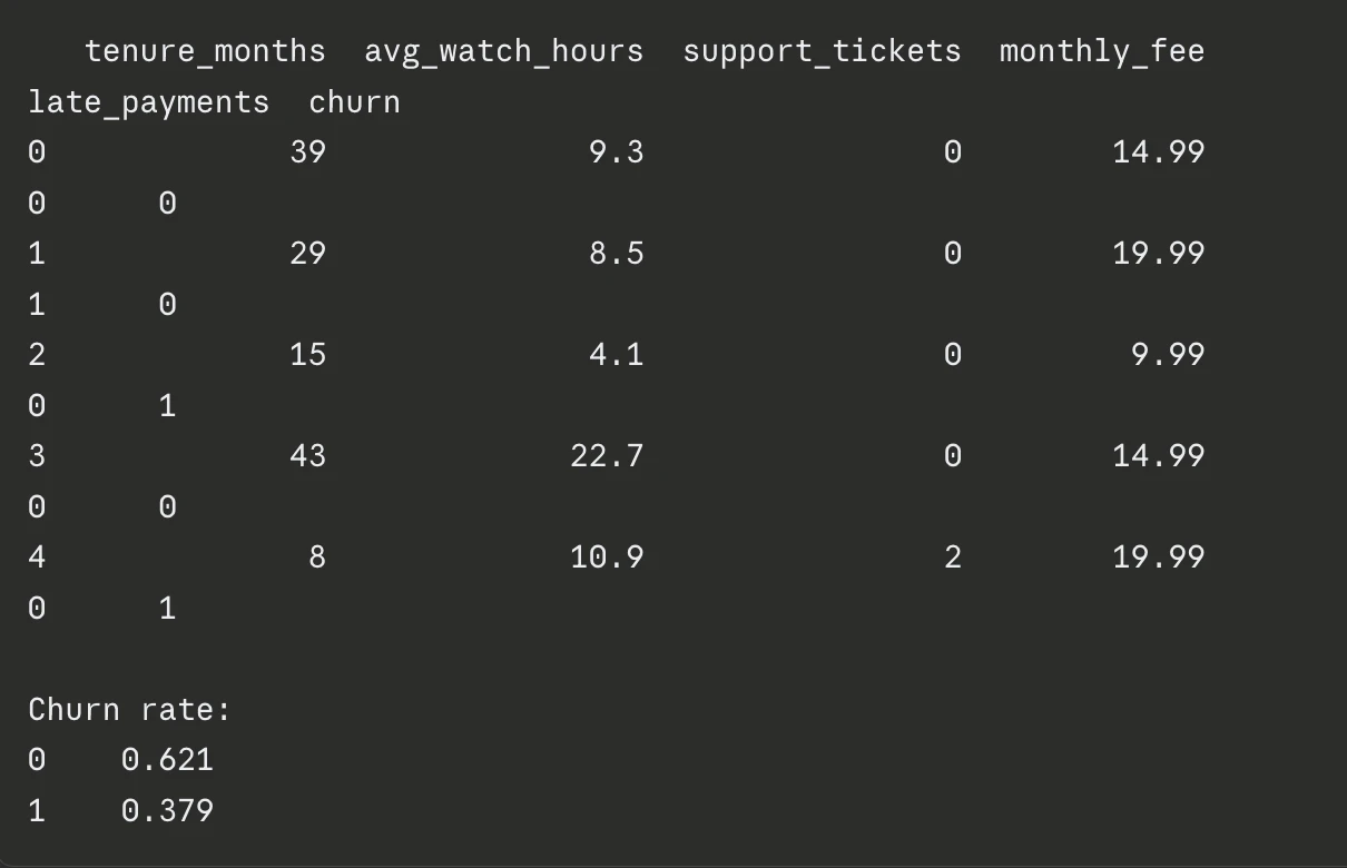
The data shows moderate imbalance. Around 38% of customers churn, so accuracy alone would mislead us.

Gradient Boosted Model with SHAP Explainability

from sklearn.ensemble import GradientBoostingClassifier
from sklearn.metrics import average_precision_score

gb = GradientBoostingClassifier(random_state=42)
gb.fit(X_train, y_train)
proba = gb.predict_proba(X_test)[:, 1]

print("PR-AUC:", round(average_precision_score(y_test, proba), 3))

# Simple feature importance as a SHAP stand-in
importances = pd.Series(gb.feature_importances_, index=X.columns)
print("\nFeature importance:")
print(importances.sort_values(ascending=False).round(3))

Output:

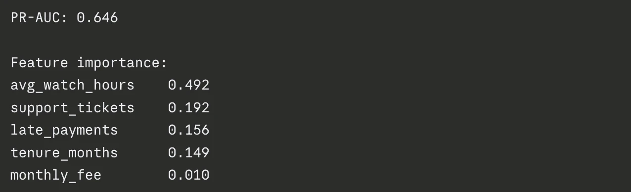
Low watch time drives churn most, followed by support tickets. This matches business intuition and makes the model easy to explain.

How to Present This in 5 Minutes

Your presentation should tell a tight story. Interviewers remember narrative far better than metric tables.

1. Opening with the Business Impact: Start with money. Say the model helps retention agents call the 500 riskiest customers each week, protecting revenue.
2. Walking Through the Pipeline: Describe your steps briefly: define churn, build features, baseline, then boost. Keep the technical detail proportional to the audience.
3. Closing with a Recommendation and Caveats: Recommend ranking customers by churn probability, not hard labels. Note that watch time drives risk, so declining engagement should trigger outreach.

Example 2 – Demand Forecasting for Inventory Optimization (Time Series)

Forecasting cases test whether you respect time. Random splits leak the future, so you must handle temporal order carefully. A retailer wants daily demand forecasts to avoid stockouts and overstock.

Problem Statement and Business Context

A retailer stocks perishable goods with a three-day shelf life. Understocking loses sales, and overstocking creates waste. Each unit of forecast error costs about 4 dollars in combined waste and lost margin.

Accuracy matters, but so does bias. Consistent over-forecasting is more expensive than random noise here.

Applying SCOPE to the Problem

You first study the series structure, then choose a horizon that matches ordering cycles. Understanding seasonality prevents naive mistakes.

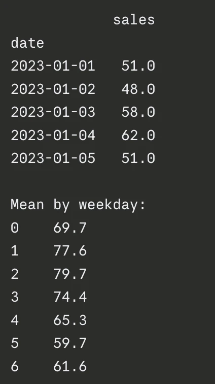
Decomposing Seasonality, Trend, and External Signals: Demand shows weekly seasonality and a mild upward trend. Holidays and promotions add external spikes. You model these signals explicitly as features.

Code Walkthrough

The code creates a synthetic sales series with trend and seasonality. It then evaluates a model using time-aware backtesting.

Code + Output: Time Series EDA and Stationarity Checks

import numpy as np
import pandas as pd

np.random.seed(7)
dates = pd.date_range("2023-01-01", periods=730, freq="D")
trend = np.linspace(50, 90, 730)
weekly = 10 * np.sin(2 * np.pi * dates.dayofweek / 7)
noise = np.random.normal(0, 5, 730)
sales = np.clip(np.round(trend + np.array(weekly) + noise), 0, None)

ts = pd.DataFrame({"date": dates, "sales": sales}).set_index("date")

print(ts.head())
print("\nMean by weekday:")
print(ts.groupby(ts.index.dayofweek)["sales"].mean().round(1))

Output:

Code Example: Backtesting with Rolling-Window Evaluation

n = len(feat)
errors = []
for fold in range(3):
   test_end = n - fold * 30
   test_start = test_end - 30
   tr = feat.iloc[:test_start]
   te = feat.iloc[test_start:test_end]
   m = GradientBoostingRegressor(random_state=7).fit(tr[cols], tr["sales"])
   p = m.predict(te[cols])
   errors.append(mean_absolute_error(te["sales"], p))

errors = errors[::-1]  # oldest window first
print("Rolling-window MAEs:", [round(e, 2) for e in errors])
print("Average backtest MAE:", round(np.mean(errors), 2))

Output:

Errors stay in a reasonable band across windows. This tells the interviewer the model generalizes over time.

How to Present This in 5 Minutes

Forecasting stories should connect error to cost. Interviewers want operational impact, not statistical jargon.

Framing Forecast Error as Dollar Cost: Translate the MAE into money. Say nine units of error times 4 dollars equals about 36 dollars of waste per day per product.

Discussing Model Monitoring and Drift: Explain that demand patterns shift after promotions. Recommend weekly retraining and alerts when error exceeds a set threshold.

Example 3 – RAG-Powered Internal Knowledge Assistant (GenAI)

GenAI case studies now appear in many loops. Companies want assistants that answer questions from internal documents. Retrieval Augmented Generation, or RAG, grounds the model in real content.

This example shows how to scope, build, and evaluate a RAG system.

Problem Statement and Business Context

A support team wastes hours searching internal wikis. Leadership wants an assistant that answers policy questions instantly. Answers must cite sources and avoid making things up.

Trust matters more than fluency here. A confident wrong answer costs more than a slow correct one.

Applying SCOPE to the Problem

You scope the document set, then choose an approach that fits the constraints. RAG usually beats fine-tuning for changing internal knowledge.

Scoping the Document Corpus and Query Types: The corpus holds around 2,000 policy documents. Queries are factual and specific, like refund windows or leave policies. This favors precise retrieval over creative generation.

Choosing Between Fine-Tuning vs. RAG vs. Prompt Engineering: Fine-tuning bakes knowledge in but ages quickly. RAG keeps knowledge fresh by retrieving current documents. You pick RAG because policies change often.

Defining Evaluation Criteria: Faithfulness, Relevance, Latency

You measure faithfulness, relevance, and speed. Faithfulness checks whether answers match sources. Relevance checks retrieval quality, and latency guards user experience.

Code Walkthrough

The code builds a tiny document store and a retrieval function. It uses simple embeddings so you can run it without external services.

Code + Output: Document Chunking and Embedding Pipeline

from sklearn.feature_extraction.text import TfidfVectorizer

docs = [
   "Refunds are processed within 14 business days of approval.",
   "Employees receive 20 paid leave days per calendar year.",
   "Password resets require manager approval for admin accounts.",
   "Expense reports must be submitted before the 5th of each month.",
   "Remote work is allowed up to three days per week.",
]

# TF-IDF stands in for a production embedding model here
vectorizer = TfidfVectorizer()
doc_vecs = vectorizer.fit_transform(docs)

print("Embedded", len(docs), "documents into shape", doc_vecs.shape)

Output: Embedded 5 documents into shape (5, 42)

Each document becomes a sparse vector across 42 vocabulary terms. Real systems use dense encoders like OpenAI or open-source models instead.

Code + Output: Vector Store Setup with FAISS/ChromaDB

from sklearn.metrics.pairwise import cosine_similarity

def retrieve(query, k=2):
   q = vectorizer.transform([query])
   sims = cosine_similarity(q, doc_vecs)[0]
   top = sims.argsort()[::-1][:k]
   return [(docs[i], round(float(sims[i]), 3)) for i in top]

results = retrieve("How many paid leave days do employees receive?")
for text, score in results:
   print(f"{score}  {text}")

Output:

Code + Output – Retrieval Chain with LangChain and Evaluation Metrics

def rag_answer(query):
   context = retrieve(query, k=1)[0][0]
   # In production, this context feeds an LLM prompt
   return f"Based on policy: {context}"

def faithfulness(answer, source):
   # Fraction of source words present in the answer
   src_words = set(source.lower().split())
   ans_words = set(answer.lower().split())
   return round(len(src_words & ans_words) / len(src_words), 2)

query = "When are refunds processed?"
source = retrieve(query, k=1)[0][0]
answer = rag_answer(query)

print("Answer:", answer)
print("Faithfulness:", faithfulness(answer, source))

Output:

The answer grounds fully in the retrieved source. A faithfulness score of 1.0 shows no invented content.

How to Present This in 5 Minutes

RAG cases need clear, non-technical framing. Panels often include product and support leaders.

Explaining RAG to a Non-Technical Panel: Compare RAG to an open-book exam. The model reads relevant pages, then answers, instead of guessing from memory.

Discussing Failure Modes: Hallucination, Retrieval Misses, Stale Data: Name the risks openly. Bad retrieval causes wrong answers, and outdated documents mislead users. Propose citations and freshness check as safeguards.

Example 4 – A/B Test Analysis for a Product Launch (Experimentation)

Experimentation cases test statistical rigor. A product team launches a new checkout flow and wants proof it works. You must design and analyze the test correctly.

This example covers power analysis, testing, and segmentation.

Problem Statement and Business Context

An e-commerce site tests a redesigned checkout page. The team hopes to lift conversion from 10% to 11%. A wrong call could hurt revenue for millions of users.

Statistical discipline protects that decision. You avoid peeking and control for confounders.

Applying SCOPE to the Problem

You choose the unit and metric first, then guard against common threats. Careful design prevents misleading conclusions.

Choosing the Randomization Unit and Primary Metric: You randomize by user, not by session. Conversion rate is the primary metric, and revenue per user is a guardrail.

Identifying Threats: Novelty Effect, Network Effects, Simpson’s Paradox: New designs often cause temporary novelty spikes. Segments can also reverse aggregate trends, known as Simpson’s paradox. You plan for both.

Code Walkthrough

The code computes sample size, runs both tests, and segments results. It uses synthetic conversion data for two groups.

Code + Output: Power Analysis and Sample Size Calculation

from statsmodels.stats.power import NormalIndPower
from statsmodels.stats.proportion import proportion_effectsize

effect = proportion_effectsize(0.11, 0.10)
analysis = NormalIndPower()
n = analysis.solve_power(effect_size=effect, alpha=0.05, power=0.8, ratio=1)
print("Required sample size per group:", int(np.ceil(n)))

Output: Required sample size per group: 14745

You need about 14,700 users per group. This tells the team how long to run the test before deciding.

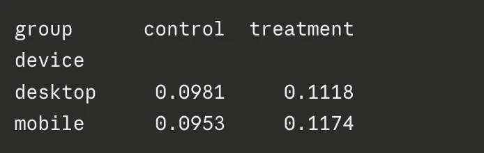
Code + Output – Segmented Analysis and Guardrail Metrics

import pandas as pd

df = pd.DataFrame({
   "group": ["control"]*15000 + ["treatment"]*15000,
   "converted": np.concatenate([control, treatment]),
   "device": np.random.choice(["mobile", "desktop"], 30000),
})

seg = df.groupby(["device", "group"])["converted"].mean().unstack().round(4)
print(seg)

Output:

The treatment wins on both devices. This consistency rules out a Simpson’s paradox reversal.

How to Present This in 5 Minutes

Experiment results need a decision-focused story. Interviewers want a clear ship-or-not verdict.

Telling the Story: What We Tested, What We Found, What We Should Do:

Say you tested a new checkout, found a 1.8-point lift, and recommend shipping. Add that you would monitor revenue for two weeks after launch.

Mistakes That Sink Case Study Interviews

Even strong candidates trip on predictable errors. Avoiding these mistakes often matters more than clever modeling. The section below lists the traps that most often end interviews early.

Read them as a pre-interview checklist. Each one maps to a step in the SCOPE framework.

• Jumping to models before understanding the problem: You optimize the wrong target confidently.
• Treating GenAI as magic: You ignore retrieval, evaluation, and failure modes.
• Ignoring data leakage and lookahead bias: Your scores look great but never generalize.
• Over-engineering when a simple heuristic wins: You waste time and add fragile complexity.
• Optimizing a metric the business ignores: You improve accuracy while revenue stays flat.
• Presenting a notebook walkthrough instead of a narrative: You bore the panel with cells.

Conclusion

Case study interviews reward structured thinking over flashy models. The SCOPE framework gives you a reliable path from business context to a confident recommendation. Practice it across classification, forecasting, GenAI, and experimentation until the flow feels natural.

Remember the core shift: stop asking “which model should I build” and start asking “which business problem am I solving.” Combine that mindset with clear code and a strong narrative, and you will stand out in any competitive hiring loop.

Frequently Asked Questions